AI & Analytics with PostgreSQL: Master Feature Engineering and Data Warehousing

💡 From Zero to Real-Time Analytics — Learn SQL the AI Way

Oct 05, 2025

🎯 Course Description

In the world of Artificial Intelligence and Machine Learning, data is everything and PostgreSQL is one of the most powerful tools to manage, clean, and prepare that data efficiently.

This course is designed for Python learners, data enthusiasts, and aspiring AI/ML professionals who want to build a strong SQL foundation using PostgreSQL, the most advanced open-source database in the world.

We start from absolute scratch understanding databases, tables, and queries and gradually build up to advanced analytical queries, window functions, feature engineering, and performance tuning.

Each chapter includes:

💻 Real-world, copy-paste runnable examples
🧠 Step-by-step explanations in plain English
📊 Mini projects linked to AI and data analytics
🧩 Exercises to build hands-on confidence

By the end, you’ll not only master SQL for data extraction and transformation you’ll learn how to bridge SQL with Python for real-time analytics, model-ready datasets, and production-grade pipelines.

🚀 Who This Course Is For

✅ Python learners stepping into AI, Data Science, or ML.
✅ Developers who want to master SQL from zero using practical examples.
✅ Data Analysts who want to transition into AI roles.
✅ AI/ML Engineers who want to design efficient feature engineering pipelines.
✅ Anyone preparing for AI/Data interviews requiring strong SQL query writing.

📚 What You’ll Learn

You’ll go from:

“I know a bit of SELECT…”
to
“I can write complex queries that feed ML models!”

Here’s a glimpse of your journey:

📍 Foundations

Understanding databases, tables, and data types
Writing queries with SELECT, WHERE, and ORDER BY
Using conditions, filters, and aliases

📍 Intermediate SQL

Aggregations (COUNT, SUM, AVG) and GROUP BY
All types of Joins and Subqueries
Common Table Expressions (CTEs)

📍 Advanced SQL

Window Functions for time-series analytics
Case statements, ranking, and rolling metrics
Data cleaning using string and date functions
JSON and semi-structured data handling

📍 Real-World AI Applications

SQL for feature engineering
Handling missing data, anomalies, and outliers
SQL + Python integration (Pandas, SQLAlchemy)
Building small ETL pipelines with PostgreSQL

🌟 Key Benefits

1️⃣ Real-World Ready

Every topic connects directly to how data scientists and AI engineers use SQL in real jobs — preparing, cleaning, and transforming data for analysis and model training.

2️⃣ Python + SQL Integration

You’ll learn to connect PostgreSQL with Python, pull datasets using pandas, and preprocess them for your AI projects or dashboards.

3️⃣ Practice Without Frustration

All examples are fully self-contained — if you copy-paste them, they just work. No missing data, no setup errors.

4️⃣ Visual Learning Approach

Each concept includes tables, outputs, and real data. You’ll understand why a query works, not just how.

5️⃣ AI-Focused SQL Mastery

This isn’t generic database training. The entire syllabus is tailored to AI/ML use cases — feature creation, time series, window analytics, and ETL workflows.

6️⃣ Practical Assignments

Each chapter ends with 10 hands-on exercises that can be solved directly in PostgreSQL — designed to reinforce learning.

7️⃣ Career-Oriented Learning Path

You’ll build the SQL confidence needed to answer data engineering, data analyst, and AI interview questions with clarity.

🧠 By the End of This Course, You’ll Be Able To:

✅ Design and query complex PostgreSQL databases.
✅ Clean, join, and transform raw data for AI/ML workflows.
✅ Write advanced SQL queries with subqueries, CTEs, and window functions.
✅ Handle JSON, arrays, and time-series data inside PostgreSQL.
✅ Integrate PostgreSQL queries directly with Python notebooks and pipelines.
✅ Debug and optimize queries for faster performance.
✅ Build complete, model-ready datasets from raw data.

🕒 Duration

6 Weeks (Self-paced, Practice-based)
Each week includes:

1 Chapter (detailed theory + 5 runnable examples + 10 exercises)
1 Practice project at the end of the module

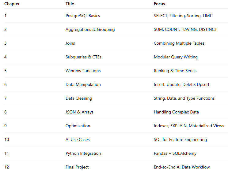
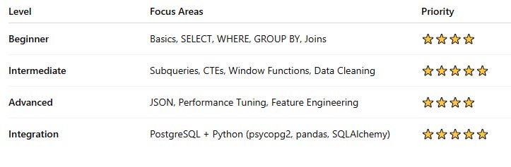
🧩 Course Structure

💼 Career Impact

After completing this course, you’ll confidently say:

“I can use SQL to build datasets for AI models and analytics — from raw data to insights.”

You’ll be ready for roles like:

Data Analyst (Python + SQL)
Data Engineer (PostgreSQL + ETL)
ML Engineer (Feature Engineering with SQL)
AI Developer (Data Prep & Integration)

🏆 Certificate of Completion

Upon completing all chapters and final project, you’ll receive a CareerByteCode Certificate showcasing your practical PostgreSQL expertise for AI and Data roles.

🚀 PostgreSQL Roadmap for AI / Data / ML Jobs

🔹Chapter 1. PostgreSQL Basics (Foundations)

Goal: Build a solid foundation in PostgreSQL syntax and structure.

What is PostgreSQL? (Architecture, Role in AI systems)
Understanding Databases, Schemas, Tables, Columns, Records
Data Types: INTEGER, NUMERIC, TEXT, BOOLEAN, DATE, TIMESTAMP
DDL, DML, DQL, DCL, TCL overview
Creating and managing databases (CREATE DATABASE, DROP DATABASE)
Creating tables with constraints (PRIMARY KEY, FOREIGN KEY, UNIQUE, NOT NULL)
SELECT, FROM, WHERE basics
Filtering data (=, <, >, <>, BETWEEN, IN, LIKE, ILIKE)
Sorting with ORDER BY
Limiting with LIMIT, OFFSET, FETCH
Aliases with AS

👉 AI Relevance: Core foundation for data extraction and manipulation before model training.

🔹Chapter 2. Aggregations & Grouping

Goal: Summarize and explore datasets effectively.

COUNT(), SUM(), AVG(), MIN(), MAX()
GROUP BY with single/multiple columns
HAVING vs WHERE
Removing duplicates with DISTINCT
Statistical queries for EDA (Exploratory Data Analysis)

👉 AI Relevance: Computing aggregates for feature engineering and EDA (mean, count, frequency features).

🔹Chapter 3. Joins (Essential for Data Engineering & AI)

Goal: Combine multiple datasets efficiently.

INNER JOIN, LEFT JOIN, RIGHT JOIN, FULL OUTER JOIN
CROSS JOIN and Cartesian products
SELF JOIN (hierarchical and recursive relationships)
Multi-table joins
Natural joins vs explicit joins

👉 AI Relevance: Combine multiple sources for dataset creation, feature enrichment, or entity linking.

🔹Chapter 4. Subqueries & CTEs (Common Table Expressions)

Goal: Create modular, readable, and optimized queries.

Subqueries in SELECT, FROM, and WHERE
Correlated vs non-correlated subqueries
EXISTS vs IN performance
Using WITH for Common Table Expressions (CTEs)
Recursive CTEs for hierarchical data

👉 AI Relevance: Break down complex queries for ETL pipelines and data preparation workflows.

🔹Chapter 5. Advanced Filtering & Window Functions

Goal: Learn analytics-level querying (critical for AI feature creation).

Conditional logic using CASE WHEN
Handling NULLs: COALESCE, NULLIF, IS NULL
Ranking functions: ROW_NUMBER(), RANK(), DENSE_RANK()
Window aggregates: SUM() OVER(), AVG() OVER()
Frame clauses: ROWS BETWEEN, RANGE BETWEEN
Lead/Lag functions for time-series (LAG(), LEAD())
Running totals, moving averages, percentiles

👉 AI Relevance: Perfect for time series modeling, rolling statistics, and trend analysis.

🔹 Chapter 6. Data Manipulation

Goal: Manage data lifecycle inside PostgreSQL.

INSERT, UPDATE, DELETE
RETURNING clause (unique to PostgreSQL)
Upsert operations using INSERT ... ON CONFLICT DO UPDATE
Bulk inserts with COPY command
Transactions with BEGIN, COMMIT, ROLLBACK

👉 AI Relevance: Managing data updates efficiently during ETL or experiment iterations.

🔹 Chapter 7. Set Operations

Goal: Combine or compare datasets for complex workflows.

UNION, UNION ALL, INTERSECT, EXCEPT
Combining datasets for training/validation splits
Deduplication with set operations

👉 AI Relevance: Useful for merging multiple datasets, or comparing model prediction results vs actuals.

🔹Chapter 8. Data Cleaning & Transformation (ETL Core)

Goal: Prepare clean, well-structured datasets for ML.

String operations: TRIM, SUBSTRING, CONCAT, UPPER, LOWER, REPLACE
Date & time functions: AGE, DATE_PART, EXTRACT, TO_CHAR, NOW()
Type conversion: CAST, ::type syntax
Pivoting data using crosstab() (from tablefunc extension)
Unpivoting / reshaping datasets
Conditional transformations using CASE

👉 AI Relevance: Critical preprocessing step before model training — clean, normalized, formatted data.

🔹 Chapter 9. JSON & Semi-Structured Data (PostgreSQL Power Feature)

Goal: Handle real-world mixed-format data efficiently.

JSON & JSONB columns
Accessing data: ->, ->>, #> operators
JSON functions: json_each(), jsonb_array_elements(), jsonb_build_object()
Querying nested structures
Storing AI/ML model metadata or configurations

👉 AI Relevance: Modern datasets often include API responses or event logs stored as JSON.

🔹Chapter 10. Array & Advanced Data Types

Goal: Work with complex and scientific data structures.

Array creation and indexing
unnest() for array flattening
Range types (int4range, numrange, daterange)
ENUMs, UUIDs, HSTORE key-value pairs

👉 AI Relevance: Helpful for storing multiple model parameters or embedding vectors.

🔹Chapter 11. Performance & Optimization

Goal: Run large queries efficiently in data pipelines.

Index types: B-tree, Hash, GIN, GiST
Creating and analyzing indexes
Query plans with EXPLAIN and EXPLAIN ANALYZE
Understanding Sequential vs Index Scan
Partitioning large tables
Materialized views
VACUUM and ANALYZE commands

👉 AI Relevance: Optimized queries mean faster ETL, real-time dashboards, and efficient training loops.

🔹Chapter 12. AI / Data-Specific Use Cases

Goal: Connect SQL knowledge directly to ML & AI workflows.

Feature engineering queries (aggregates, ratios, time-based deltas)
Time-series transformations (lags, moving windows)
Anomaly detection with SQL-based thresholds
Missing value detection (COUNT(NULL), COALESCE)
Deduplication and data consistency checks
Statistical summaries with SQL
Creating feature stores in PostgreSQL

🔹Chapter 13. PostgreSQL with Python (Integration)

Goal: Combine PostgreSQL and Python seamlessly for end-to-end data work.

Connecting using psycopg2 or SQLAlchemy
Reading queries into Pandas DataFrames (pd.read_sql())
Writing model outputs back to PostgreSQL
Using COPY for fast bulk inserts from Python
Building ETL pipelines (Airflow + Postgres + Pandas)
Query automation via Jupyter or scripts

👉 AI Relevance: The bridge between SQL and ML model development.

🔹Chapter 14. Data Warehousing & Analytical Extensions

Goal: Handle enterprise-scale analytics.

Understanding extensions like TimescaleDB (for time series)
CUBE, ROLLUP, and GROUPING SETS
PostgreSQL partitioning for analytical datasets
Integration with BI tools (Power BI, Tableau, Metabase)
Using FDW (Foreign Data Wrapper) for external data access

👉 AI Relevance: Scaling SQL analysis for production AI data pipelines.

✅ Summary: What You Must Master for AI Jobs

🔗 Recommended Tools for Practice

PostgreSQL (install locally or use Docker)
pgAdmin / DBeaver (GUI tools)
Jupyter Notebook + SQLAlchemy (Python integration)
Kaggle Datasets + PostgreSQL (real-world AI practice)

Chapter 1 — PostgreSQL Basics (Foundations)

What you’ll learn in this chapter (in one sentence)

You’ll learn what PostgreSQL is, the basic building blocks of a database (databases → schemas → tables → rows/columns), how to write simple SELECT queries, filter results, sort them, limit rows, and use column aliases — all explained in plain language.

Layman explanations (super simple)

What is PostgreSQL?
PostgreSQL (Postgres) is a program that stores data for you (like a super-organized filing cabinet). You ask it for data using SQL (a language); it gives the data back.
Database vs Schema vs Table vs Row vs Column
- Database: A whole filing cabinet.
- Schema: A drawer inside the cabinet (helps organize).
- Table: A file folder in the drawer (holds similar records).
- Row: One sheet of paper in the folder (a single item/record).
- Column: A labeled line on the sheet (a specific attribute, like “name” or “age”).
Primary Key
A column that uniquely identifies each row — like a unique ID number on each sheet.
Foreign Key
A column that points to a primary key in another table — like a reference to another file.
Data types
Tells Postgres what kind of info a column holds: INTEGER (numbers), TEXT (words), BOOLEAN (true/false), TIMESTAMP (date & time), etc.
DDL / DML / DQL
- DDL (Data Definition Language): Commands that create or change the structure (e.g., CREATE TABLE).
- DML (Data Manipulation Language): Commands that modify data (e.g., INSERT, UPDATE, DELETE).
- DQL (Data Query Language): Commands that read data (mostly SELECT).
SELECT, FROM, WHERE
- SELECT lists which columns you want.
- FROM says which table.
- WHERE filters rows (gives conditions).
Filtering operators
Use = (equal), <, >, <> (not equal), BETWEEN, IN (in a set), LIKE (pattern matching).
ORDER BY
Sort the results (e.g., newest first or lowest price first).
LIMIT / OFFSET
Only take the first N rows (LIMIT), or skip some and then take (OFFSET).
Aliases (AS)
Rename columns or tables within your query to make output cleaner or queries shorter.

Practical Examples (each is copy-paste runnable)

Note: Each example starts with DROP TABLE IF EXISTS so you can re-run freely.

Example 1 — Basic SELECT and creating a table

Scenario: A tiny people table. Show selected columns.

-- Example 1: basic SELECT
DROP TABLE IF EXISTS ex1_people;

CREATE TABLE ex1_people (
  person_id SERIAL PRIMARY KEY,
  full_name TEXT NOT NULL,
  age INTEGER,
  city TEXT
);

INSERT INTO ex1_people (full_name, age, city) VALUES
(’Anita Sharma’, 28, ‘Brussels’),
(’Mark Johnson’, 35, ‘London’),
(’Sana Ali’, 22, ‘Amsterdam’),
(’Tom Lee’, NULL, ‘Berlin’);  -- Tom’s age unknown

-- 1) select all columns
SELECT * FROM ex1_people;

-- 2) select specific columns
SELECT full_name, city FROM ex1_people;

-- 3) rename a column in output
SELECT full_name AS name, age AS years FROM ex1_people;

What you learned: how to create a table, insert rows, and fetch all or specific columns. NULL means unknown.

Example 2 — Filtering with WHERE and operators

Scenario: Products table — use =, <, >, <>, BETWEEN, IN, LIKE, ILIKE.

-- Example 2: filtering
DROP TABLE IF EXISTS ex2_products;
CREATE TABLE ex2_products (
  product_id SERIAL PRIMARY KEY,
  name TEXT NOT NULL,
  price NUMERIC(8,2),
  category TEXT
);

INSERT INTO ex2_products (name, price, category) VALUES
(’Coffee Beans’, 12.50, ‘Beverage’),
(’Green Tea’, 8.00, ‘Beverage’),
(’Notebook A4’, 3.25, ‘Stationery’),
(’Premium Notebook’, 7.50, ‘Stationery’),
(’Espresso Machine’, 120.00, ‘Appliance’);

-- Equal
SELECT * FROM ex2_products WHERE category = ‘Beverage’;

-- Not equal
SELECT * FROM ex2_products WHERE price <> 12.50;

-- Greater than / Less than
SELECT name, price FROM ex2_products WHERE price > 10.00;

-- BETWEEN
SELECT name, price FROM ex2_products WHERE price BETWEEN 5 AND 50;

-- IN (matches any of a list)
SELECT * FROM ex2_products WHERE category IN (’Beverage’, ‘Appliance’);

-- LIKE (pattern; % means any chars)
SELECT * FROM ex2_products WHERE name LIKE ‘%Notebook%’;

-- ILIKE (case-insensitive)
SELECT * FROM ex2_products WHERE name LIKE ‘coffee%’;

What you learned: common filters and pattern matching (case sensitive LIKE, case-insensitive ILIKE).

Example 3 — ORDER BY, LIMIT, OFFSET

Scenario: Students leaderboard — sort by score and paginate.

-- Example 3: order, limit, offset
DROP TABLE IF EXISTS ex3_students;
CREATE TABLE ex3_students (
  student_id SERIAL PRIMARY KEY,
  name TEXT,
  score INTEGER,
  taken_at TIMESTAMP
);

INSERT INTO ex3_students (name, score, taken_at) VALUES
(’Aisha’, 92, ‘2025-01-05 10:00’),
(’Ben’, 85, ‘2025-01-06 11:30’),
(’Carla’, 78, ‘2025-01-04 09:20’),
(’Derek’, 92, ‘2025-01-07 14:00’),
(’Eve’, 68, ‘2025-01-03 08:00’);

-- Sort by highest score first, newest attempt first
SELECT name, score, taken_at
FROM ex3_students
ORDER BY score DESC, taken_at DESC;

-- Only top 3
SELECT name, score FROM ex3_students ORDER BY score DESC LIMIT 3;

-- Pagination: skip first 2, show next 2
SELECT name, score FROM ex3_students ORDER BY score DESC LIMIT 2 OFFSET 2;

What you learned: ordering, limiting results and simple pagination with LIMIT and OFFSET.

Example 4 — Aliases, expressions, and casting

Scenario: Employee salaries; show monthly pay and format.

-- Example 4: aliases, calculation, type casting
DROP TABLE IF EXISTS ex4_staff;
CREATE TABLE ex4_staff (
  staff_id SERIAL PRIMARY KEY,
  name TEXT,
  annual_salary NUMERIC(12,2),
  join_date DATE
);

INSERT INTO ex4_staff (name, annual_salary, join_date) VALUES
(’Ramesh’, 60000.00, ‘2020-06-15’),
(’Julia’, 48000.50, ‘2021-09-01’),
(’Liam’, 72000.00, ‘2019-03-10’);

-- Calculate monthly salary (simple division), show with alias
SELECT name,
       annual_salary,
       (annual_salary / 12) AS monthly_salary
FROM ex4_staff;

-- Round monthly salary to 2 decimals and show as text label
SELECT name,
       annual_salary,
       ROUND(annual_salary / 12, 2) AS monthly_salary_rounded,
       (ROUND(annual_salary / 12, 2))::TEXT || ‘ EUR/month’ AS pay_label
FROM ex4_staff;

What you learned: you can do math in SELECT, assign a friendly column name with AS, and cast results to text for readable labels.

Example 5 — DISTINCT and basic uniqueness check

Scenario: Orders with cities — find unique cities, and count distinct.

-- Example 5: DISTINCT
DROP TABLE IF EXISTS ex5_orders;
CREATE TABLE ex5_orders (
  order_id SERIAL PRIMARY KEY,
  customer TEXT,
  city TEXT,
  amount NUMERIC(8,2)
);

INSERT INTO ex5_orders (customer, city, amount) VALUES
(’Anna’, ‘Brussels’, 34.50),
(’Ben’, ‘Brussels’, 15.00),
(’Carmen’, ‘Antwerp’, 44.00),
(’David’, ‘Ghent’, 21.25),
(’Ella’, ‘Antwerp’, 99.99);

-- Get unique cities
SELECT DISTINCT city FROM ex5_orders;

-- Count unique cities
SELECT COUNT(DISTINCT city) AS unique_city_count FROM ex5_orders;

-- Distinct combinations (customer+city)
SELECT DISTINCT customer, city FROM ex5_orders;

What you learned: DISTINCT removes duplicates from the result set.

Example 6 — Basic table constraints (NOT NULL, UNIQUE, PRIMARY KEY)

Scenario: Simple contacts table demonstrating constraints and safe inserts.

-- Example 6: constraints
DROP TABLE IF EXISTS ex6_contacts;
CREATE TABLE ex6_contacts (
  contact_id SERIAL PRIMARY KEY,
  email TEXT UNIQUE NOT NULL,
  name TEXT NOT NULL,
  phone TEXT
);

-- valid insert
INSERT INTO ex6_contacts (email, name, phone) VALUES
(’alice@example.com’,’Alice’,’+32-2-555-0100’),
(’bob@example.com’,’Bob’,NULL);

-- Trying to insert NULL into email or duplicate email would fail:
-- (these lines are commented out so script runs; try them manually)
-- INSERT INTO ex6_contacts (email, name) VALUES (NULL, ‘Bad’); -- error due to NOT NULL
-- INSERT INTO ex6_contacts (email, name) VALUES (’alice@example.com’,’Duplicate’); -- UNIQUE violation

SELECT * FROM ex6_contacts;

What you learned: constraints enforce rules — NOT NULL, UNIQUE, PRIMARY KEY keep data valid. I commented the failing inserts so the script runs cleanly; try them yourself to see the errors.

Quick troubleshooting tips

If you see relation “ex1_people” does not exist, make sure you executed the CREATE TABLE block first.
If an INSERT fails with duplicate key value violates unique constraint, it means you tried to insert a value that must be unique (like an email or primary key).
Use \d tablename in psql to inspect table structure.

10 Exercises (practice tasks for Chapter 1)

Try these on your own. For each exercise write SQL to solve it.

Make a books table with columns book_id (PK), title, author, price. Insert 6 books, then select all books cheaper than 20.
Create a visitors table with visitor_id, name, visit_date. Insert 5 rows. Select rows where visit_date is after ‘2025-01-01’.
Filter by multiple conditions: Using a table ex2_products-style, select products where category = ‘Stationery’ and price < 5.
Case-insensitive search: Create a users table with usernames in mixed case. Use a query to find username starting with ‘jo’ regardless of case.
Top-N: Create a scores table, insert 8 rows and return top 3 scorers.
Aliases and calculations: Make a sales table with unit_price and quantity. Show total = unit_price * quantity with alias order_total.
Distinct usage: Create an events table with event names and cities. List all distinct cities.
Constraint test: Create a members table where email must be unique and name not null. Try inserting duplicates to see the error. (Explain what happened.)
Limit + Offset: Create a messages table and return rows 6–10 ordered by timestamp (simulate pagination).
Explain why NULL matters: Create a table with a column allowed to be NULL. Insert a row with NULL and another without. Show how WHERE column = ‘something’ ignores the NULL row, but WHERE column IS NULL picks it up.

Chapter 2 — Aggregations & Grouping

(Plain-English explanations + very detailed examples you can copy-paste + 10 hands-on exercises)

Bavi — this chapter teaches how to summarize and roll up data: counts, sums, averages, min/max, and how to group rows into buckets (by product, by day, by city) so you can get the high-level numbers data scientists need for EDA and feature engineering.

What you’ll learn in plain English

Aggregate functions are small math tools Postgres gives you: COUNT, SUM, AVG, MIN, MAX. They take many rows and return one number (e.g., total sales).
GROUP BY collects rows into buckets (e.g., one bucket per product) so you can run aggregates per bucket.
HAVING filters buckets after aggregation (e.g., show only products whose total sales exceed €500).
COUNT(*) vs COUNT(column) — COUNT(*) counts rows; COUNT(column) only counts non-NULL values.
COUNT(DISTINCT ...) counts unique values inside each group.
FILTER (Postgres feature) lets you run conditional aggregates in the same query (e.g., count purchases vs refunds).
DATE_TRUNC is handy to group timestamps by month/week/day. Very useful for time-series features.

All examples below are fully self-contained (they DROP then CREATE tables and INSERT data). Copy-paste any single example into your psql, pgAdmin, DBeaver, or other Postgres client and it will run.

Example 1 — Simple aggregates: COUNT, SUM, AVG, MIN, MAX

Goal: See the basic aggregate functions in action on a small transactions table.

-- EX1: Basic aggregates
DROP TABLE IF EXISTS ex1_transactions;
CREATE TABLE ex1_transactions (
  txn_id   SERIAL PRIMARY KEY,
  user_id  INTEGER,
  amount   NUMERIC(10,2),
  txn_time TIMESTAMP
);

INSERT INTO ex1_transactions (user_id, amount, txn_time) VALUES
(1, 12.50, ‘2025-01-01 09:10’),
(2, 7.00,  ‘2025-01-01 10:00’),
(1, 5.25,  ‘2025-01-02 11:15’),
(3, NULL,  ‘2025-01-03 12:00’), -- failed / missing amount
(2, 20.00, ‘2025-01-04 13:00’),
(4, 100.00,’2025-01-05 14:30’);

-- a) total number of transactions (rows)
SELECT COUNT(*) AS total_transactions FROM ex1_transactions;

-- b) total amount of all transactions (NULL values ignored by SUM)
SELECT SUM(amount) AS total_amount FROM ex1_transactions;

-- c) average amount per transaction (NULLs ignored)
SELECT AVG(amount) AS avg_amount FROM ex1_transactions;

-- d) smallest and largest transaction amounts
SELECT MIN(amount) AS smallest, MAX(amount) AS largest FROM ex1_transactions;

-- e) combine them in one row for an overview
SELECT
  COUNT(*) AS total_rows,
  COUNT(amount) AS rows_with_amount,
  SUM(amount) AS sum_amount,
  AVG(amount) AS avg_amount,
  MIN(amount) AS min_amount,
  MAX(amount) AS max_amount
FROM ex1_transactions;

Why this matters (layman): COUNT tells you how many rows; SUM adds numbers; AVG finds the mean; MIN and MAX show extremes. Notice SUM and AVG ignore NULL amounts — that prevents broken math when some rows are missing data.

Example 2 — GROUP BY a single column: totals per category

Goal: Group sales by category to see which categories sell the most.

-- EX2: Group by category (sales totals and counts)
DROP TABLE IF EXISTS ex2_category_sales;
CREATE TABLE ex2_category_sales (
  sale_id  SERIAL PRIMARY KEY,
  product  TEXT,
  category TEXT,
  qty      INTEGER,
  unit_price NUMERIC(8,2)
);

INSERT INTO ex2_category_sales (product, category, qty, unit_price) VALUES
(’Espresso Beans’,’Beverage’, 10, 12.50),
(’Green Tea’,’Beverage’, 5, 8.00),
(’Notebook A4’,’Stationery’, 50, 3.25),
(’Premium Notebook’,’Stationery’, 20, 7.50),
(’Espresso Machine’,’Appliance’, 2, 120.00),
(’Mug’,’Merch’, 100, 4.00),
(’Sticker Pack’,’Merch’, 200, 1.50);

-- Calculate total sales per category and number of items sold
SELECT
  category,
  SUM(qty * unit_price) AS total_revenue,
  SUM(qty) AS total_units_sold,
  COUNT(*) AS number_of_line_items
FROM ex2_category_sales
GROUP BY category
ORDER BY total_revenue DESC;

What you see: Each category becomes one row; inside that row we compute SUM(qty * unit_price) to get revenue for that category. GROUP BY is how we “fold” rows into buckets.

Example 3 — GROUP BY multiple columns and time bucketing (DATE_TRUNC)

Goal: For each city and each month, compute total revenue — extremely useful for time-series features.

-- EX3: Group by city and month (time bucketing)
DROP TABLE IF EXISTS ex3_orders;
CREATE TABLE ex3_orders (
  order_id   SERIAL PRIMARY KEY,
  customer   TEXT,
  city       TEXT,
  amount     NUMERIC(10,2),
  order_ts   TIMESTAMP
);

INSERT INTO ex3_orders (customer, city, amount, order_ts) VALUES
(’Anna’,’Brussels’, 34.50, ‘2025-01-05 10:00’),
(’Ben’,’Brussels’, 15.00, ‘2025-01-06 12:00’),
(’Carmen’,’Antwerp’, 44.00, ‘2025-01-20 09:00’),
(’David’,’Ghent’, 21.25, ‘2025-02-02 11:00’),
(’Ella’,’Antwerp’, 99.99, ‘2025-02-10 14:00’),
(’Fahad’,’Brussels’, 12.00, ‘2025-02-12 16:00’),
(’Gina’,’Brussels’, 60.00, ‘2025-03-01 10:30’);

-- Group by city and month
SELECT
  city,
  DATE_TRUNC(’month’, order_ts) AS month,
  COUNT(*) AS orders_count,
  SUM(amount) AS month_revenue,
  AVG(amount) AS avg_order_value
FROM ex3_orders
GROUP BY city, DATE_TRUNC(’month’, order_ts)
ORDER BY month, city;

Why this is handy: DATE_TRUNC(’month’, order_ts) converts a timestamp to the month (e.g., ‘2025-02-01 00:00:00’) so months become grouping keys. Grouping by more than one column (city + month) gives a grid of metrics you can turn into time-series features for ML.

Example 4 — HAVING vs WHERE: filter groups (correct way)

Goal: Show how to keep only buckets that meet a condition (like categories with total revenue > 100).

-- EX4: HAVING to filter groups
DROP TABLE IF EXISTS ex4_sales;
CREATE TABLE ex4_sales (
  id SERIAL PRIMARY KEY,
  category TEXT,
  amount   NUMERIC(8,2)
);

INSERT INTO ex4_sales (category, amount) VALUES
(’Beverage’, 12.50),
(’Beverage’, 8.00),
(’Stationery’, 3.25),
(’Stationery’, 7.50),
(’Appliance’, 120.00),
(’Merch’, 4.00),
(’Merch’, 1.50),
(’Merch’, 150.00);

-- WRONG: this would fail because WHERE cannot use aggregates (commented)
-- SELECT category, SUM(amount) FROM ex4_sales WHERE SUM(amount) > 100 GROUP BY category;

-- RIGHT: use HAVING to filter groups after aggregation
SELECT
  category,
  SUM(amount) AS total_revenue
FROM ex4_sales
GROUP BY category
HAVING SUM(amount) > 100
ORDER BY total_revenue DESC;

-- Alternative: using a subquery with WHERE (also valid)
SELECT category, total_revenue FROM (
  SELECT category, SUM(amount) AS total_revenue
  FROM ex4_sales
  GROUP BY category
) t
WHERE total_revenue > 100;

Layman explanation: WHERE filters individual rows before grouping. HAVING filters the grouped results after you compute SUM/AVG/etc. Use HAVING when your condition uses aggregated numbers.

Example 5 — COUNT(DISTINCT), FILTER clause, and conditional aggregates

Goal: Count unique users and compute purchase-only sums in the same grouped query.

-- EX5: DISTINCT counts and FILTER (Postgres)
DROP TABLE IF EXISTS ex5_user_events;
CREATE TABLE ex5_user_events (
  event_id   SERIAL PRIMARY KEY,
  user_id    INTEGER,
  event_type TEXT,     -- ‘view’, ‘add_to_cart’, ‘purchase’, ‘refund’
  amount     NUMERIC(10,2),
  event_ts   TIMESTAMP
);

INSERT INTO ex5_user_events (user_id, event_type, amount, event_ts) VALUES
(1, ‘view’, NULL,  ‘2025-03-01 09:00’),
(1, ‘add_to_cart’, NULL, ‘2025-03-01 09:05’),
(1, ‘purchase’, 20.00, ‘2025-03-01 09:06’),
(2, ‘view’, NULL, ‘2025-03-01 10:00’),
(2, ‘purchase’, 15.00, ‘2025-03-02 11:00’),
(3, ‘view’, NULL, ‘2025-03-02 12:00’),
(3, ‘purchase’, 7.50, ‘2025-03-02 12:05’),
(3, ‘refund’, -7.50, ‘2025-03-03 13:00’),
(4, ‘purchase’, 100.00, ‘2025-03-04 14:00’),
(4, ‘purchase’, 50.00, ‘2025-03-05 15:00’);

-- Aggregate example: per-day summary
SELECT
  DATE(event_ts) AS day,
  COUNT(*) AS total_events,
  COUNT(DISTINCT user_id) AS unique_users,
  COUNT(*) FILTER (WHERE event_type = ‘purchase’) AS purchase_events,
  SUM(amount) FILTER (WHERE event_type = ‘purchase’) AS purchase_amount,
  SUM(amount) FILTER (WHERE event_type = ‘refund’) AS refund_amount
FROM ex5_user_events
GROUP BY DATE(event_ts)
ORDER BY day;

Plain take-away: COUNT(DISTINCT user_id) gives number of unique users. FILTER (WHERE ...) is a clean Postgres way to say “run this aggregate but only for rows that match this condition” — very useful to compute multiple conditional counts/sums in a single query.

Example 6 — NULLs, COUNT(*) vs COUNT(col), and grouping NULLs with COALESCE

Goal: Understand how NULL affects aggregates and how to group NULL values cleanly.

-- EX6: NULL handling in aggregates
DROP TABLE IF EXISTS ex6_feedback;
CREATE TABLE ex6_feedback (
  fb_id    SERIAL PRIMARY KEY,
  product_id INTEGER,  -- can be NULL (feedback not tied to product)
  rating   INTEGER,    -- 1..5 or NULL if not rated
  comments TEXT
);

INSERT INTO ex6_feedback (product_id, rating, comments) VALUES
(1, 5, ‘Great’),
(1, 4, ‘Good’),
(NULL, 3, ‘General feedback’),
(2, NULL, ‘No rating’),
(2, 2, ‘Poor’),
(NULL, NULL, ‘Anonymous note’);

-- Counts:
SELECT
  COUNT(*) AS total_rows,
  COUNT(product_id) AS rows_with_product_id,
  COUNT(rating) AS rows_with_rating,
  COUNT(DISTINCT product_id) AS distinct_products_referenced
FROM ex6_feedback;

-- Group by product_id will put NULLs in a distinct bucket.
-- Use COALESCE to label NULL product_id as ‘unknown’ when grouping.
SELECT
  COALESCE(product_id::TEXT, ‘unknown’) AS product_label,
  COUNT(*) AS feedback_count,
  AVG(rating) AS avg_rating
FROM ex6_feedback
GROUP BY COALESCE(product_id::TEXT, ‘unknown’);

Key point for beginners: COUNT(*) counts every row. COUNT(product_id) ignores rows where product_id is NULL. When grouping, NULL is a real bucket — use COALESCE to make it human-friendly (e.g., ‘unknown’).

Quick practical tips (layman)

If you want totals per day/week/month: use DATE_TRUNC(’day’|’week’|’month’, timestamp_col) in GROUP BY.
Use ORDER BY on aggregated columns (e.g., ORDER BY SUM(amount) DESC) to find top buckets.
To filter groups by their aggregate value use HAVING.
Use COUNT(DISTINCT ...) to know how many unique users, products, etc.
If you need multiple conditional aggregates (e.g., purchases vs refunds), use FILTER — it’s clearer than SUM(CASE WHEN ...). (Both work.)

10 Exercises — practice (all should be solved in PostgreSQL)

Try to write the SQL for each. If you want, I’ll provide the full runnable solution scripts afterwards.

Total revenue & average order value: Create an orders table (order_id, customer_id, amount, order_ts). Insert 12 rows across two months. Write a query that returns the total revenue and AVG order amount for the entire dataset.
Revenue per product: Create product_sales(product, category, qty, unit_price) (insert 20 rows across 4 categories). Return total revenue and units sold per category, sorted by revenue descending.
Monthly active users: Create events(user_id, event_type, event_ts) where event_type can be ‘view’ or ‘purchase’. Write a query that shows month (YYYY-MM) and number of unique users who made a purchase in that month.
Top 3 customers: Using an orders table (customer_id, amount), return the top 3 customers by total spending (customer_id and total_spent).
Filter groups with HAVING: Create a sales table and find categories whose total sales amount is at least 500. Use HAVING.
Conditional aggregates: Create events with types ‘purchase’ and ‘refund’. For each day, compute: total_events, purchase_count, refund_count, purchase_amount, refund_amount. Use FILTER or SUM(CASE WHEN ...).
Count vs Count(column): Build a responses table with a nullable rating and show COUNT(*) vs COUNT(rating) and explain the difference in one sentence (as a SQL comment).
Group by multiple columns: Using an orders table with city and order_ts, compute city, month, orders_count, total_amount grouped by city and month for the last 90 days.
Top-N per group (advanced): For sales(employee_id, region, sale_amount), find the highest sale per region (region + employee_id + sale_amount). (Hint: use ROW_NUMBER() over partition — this crosses into window functions but is very useful. If you prefer not to use window functions yet, use a subquery per region.)
Distinct counts in groups: Create a visits(user_id, page, visit_ts) table. For each page, compute how many unique users visited it and the total visits. Sort pages by unique users descending.

Chapter 3 — Joins (Very plain-English + runnable examples + 10 exercises)

Alright Bavi — here’s Chapter 3: Joins. I’ll explain every concept like you’re reading a friendly cheat-sheet, then provide at least 5 fully runnable examples (each example drops/creates its own tables and inserts data so you can copy/paste and run). Every example is followed by a short plain-language explanation. At the end are 10 exercises to practice.

What is a JOIN? (super simple)

A join lets you combine rows from two (or more) tables into a single row in the result — based on some matching rule.
Think of two lists: one is people, another is their phones. A join answers questions like “show me each person and their phone” or “show all people even if they don’t have a phone”.

Key idea: a join picks rows from Table A and rows from Table B and sticks them together when a matching condition is true (usually when an id in A equals an id in B).

Types of joins — in one line each

INNER JOIN: Only rows that have matches in both tables. (Think: intersection.)
LEFT (LEFT OUTER) JOIN: All rows from the left table; matching rows from right when available; otherwise NULLs for right columns. (Think: everything on the left, bring matching right info.)
RIGHT (RIGHT OUTER) JOIN: All rows from the right table; matching left when available. (Less used but symmetric to LEFT.)
FULL OUTER JOIN: All rows from both tables; where no match exists, fill with NULLs. (Union of left and right with matching combined.)
CROSS JOIN: Cartesian product — every row from A paired with every row from B (be careful: can explode).
SELF JOIN: A table joined to itself (useful for hierarchies).
Multi-table joins: Chain joins across several tables to build richer rows.

Syntax basics

SELECT ... FROM A INNER JOIN B ON A.key = B.key;
LEFT JOIN and RIGHT JOIN work the same but preserve rows from one side.
You can use USING(col) when both tables have the same column name for the join key — this avoids repeating ON A.col = B.col.

Example 1 — INNER JOIN (basic)

-- EX1: INNER JOIN basic
DROP TABLE IF EXISTS ex1_customers;
DROP TABLE IF EXISTS ex1_orders;

CREATE TABLE ex1_customers (
  customer_id SERIAL PRIMARY KEY,
  name TEXT,
  city TEXT
);

CREATE TABLE ex1_orders (
  order_id SERIAL PRIMARY KEY,
  customer_id INTEGER REFERENCES ex1_customers(customer_id),
  amount NUMERIC(8,2),
  order_ts TIMESTAMP
);

INSERT INTO ex1_customers (name, city) VALUES
(’Anita’, ‘Brussels’),
(’Ben’, ‘London’),
(’Carmen’, ‘Antwerp’);

INSERT INTO ex1_orders (customer_id, amount, order_ts) VALUES
(1, 34.50, ‘2025-01-05 10:00’),
(1, 15.00, ‘2025-01-06 12:00’),
(3, 44.00, ‘2025-01-20 09:00’);

-- Inner join: only customers who have orders
SELECT c.customer_id, c.name, o.order_id, o.amount, o.order_ts
FROM ex1_customers c
INNER JOIN ex1_orders o
  ON c.customer_id = o.customer_id
ORDER BY c.customer_id, o.order_id;

Plain take-away: Inner join shows only customers that have orders. Anita and Carmen appear because they have orders; Ben does not because he has none.

Example 2 — LEFT JOIN (include unmatched left rows)

-- EX2: LEFT JOIN shows all customers, even if no orders
DROP TABLE IF EXISTS ex2_customers;
DROP TABLE IF EXISTS ex2_orders;

CREATE TABLE ex2_customers (
  customer_id SERIAL PRIMARY KEY,
  name TEXT
);

CREATE TABLE ex2_orders (
  order_id SERIAL PRIMARY KEY,
  customer_id INTEGER,
  amount NUMERIC(8,2)
);

INSERT INTO ex2_customers (name) VALUES
(’Ali’),
(’Beth’),
(’Cheng’);

INSERT INTO ex2_orders (customer_id, amount) VALUES
(1, 10.00),
(1, 5.00),
(3, 100.00);

-- Left join: all customers; orders when available
SELECT c.customer_id, c.name, o.order_id, o.amount
FROM ex2_customers c
LEFT JOIN ex2_orders o
  ON c.customer_id = o.customer_id
ORDER BY c.customer_id;

Plain take-away: Beth (customer_id 2) will appear with NULLs for order fields — left join preserves all left-table rows even if no match on the right.

Example 3 — RIGHT JOIN and FULL OUTER JOIN

-- EX3: RIGHT JOIN and FULL OUTER JOIN
DROP TABLE IF EXISTS ex3_employees;
DROP TABLE IF EXISTS ex3_departments;

CREATE TABLE ex3_employees (
  emp_id SERIAL PRIMARY KEY,
  name TEXT,
  dept_id INTEGER
);

CREATE TABLE ex3_departments (
  dept_id SERIAL PRIMARY KEY,
  dept_name TEXT
);

INSERT INTO ex3_employees (name, dept_id) VALUES
(’Ravi’, 1),
(’Mia’, 2),
(’Noah’, NULL);  -- Noah not assigned

INSERT INTO ex3_departments (dept_name) VALUES
(’Engineering’),
(’HR’),
(’Legal’);  -- Legal has no employees yet

-- Right join: all departments, employees info when present
SELECT e.emp_id, e.name, d.dept_id, d.dept_name
FROM ex3_employees e
RIGHT JOIN ex3_departments d
  ON e.dept_id = d.dept_id
ORDER BY d.dept_id;

-- Full outer join: everything from both sides
SELECT e.emp_id, e.name, d.dept_id, d.dept_name
FROM ex3_employees e
FULL OUTER JOIN ex3_departments d
  ON e.dept_id = d.dept_id
ORDER BY COALESCE(d.dept_id, 999), e.emp_id;

Plain take-away:

RIGHT JOIN keeps all departments; Engineering and HR will show matching employees and Legal will show NULL employee columns.
FULL OUTER JOIN shows Noah (employee with no dept) and Legal (dept with no employees) in the same result.

Example 4 — CROSS JOIN (cartesian product)

-- EX4: CROSS JOIN can blow up rows, use with care
DROP TABLE IF EXISTS ex4_colors;
DROP TABLE IF EXISTS ex4_sizes;

CREATE TABLE ex4_colors (color TEXT);
CREATE TABLE ex4_sizes (size TEXT);

INSERT INTO ex4_colors VALUES (’Red’), (’Blue’);
INSERT INTO ex4_sizes VALUES (’S’), (’M’), (’L’);

-- Cross join: every color combined with every size (2 * 3 = 6 rows)
SELECT color, size FROM ex4_colors CROSS JOIN ex4_sizes ORDER BY color, size;

Plain take-away: CROSS JOIN pairs every row from first table with every row from second. Useful for generating combinations, but be careful with big tables.

Example 5 — SELF JOIN (table joined to itself)

-- EX5: SELF JOIN for manager-employee relationships
DROP TABLE IF EXISTS ex5_people;

CREATE TABLE ex5_people (
  person_id SERIAL PRIMARY KEY,
  name TEXT,
  manager_id INTEGER  -- points to person_id
);

INSERT INTO ex5_people (name, manager_id) VALUES
(’CEO’, NULL),
(’Alice’, 1),
(’Bob’, 1),
(’Charlie’, 2),
(’Diana’, 2);

-- Self join: show employee + their manager name
SELECT e.person_id AS emp_id, e.name AS employee,
       m.person_id AS mgr_id, m.name AS manager
FROM ex5_people e
LEFT JOIN ex5_people m
  ON e.manager_id = m.person_id
ORDER BY e.person_id;

Plain take-away: Self join treats the table as two roles (employee and manager) so we can display relationships stored as IDs in the same table.

Example 6 — Multi-table joins (chain joins) + USING

-- EX6: Multi-table join (orders -> customers -> shipments)
DROP TABLE IF EXISTS ex6_customers;
DROP TABLE IF EXISTS ex6_orders;
DROP TABLE IF EXISTS ex6_shipments;

CREATE TABLE ex6_customers (
  customer_id SERIAL PRIMARY KEY,
  name TEXT
);

CREATE TABLE ex6_orders (
  order_id SERIAL PRIMARY KEY,
  customer_id INTEGER REFERENCES ex6_customers(customer_id),
  amount NUMERIC(8,2)
);

CREATE TABLE ex6_shipments (
  shipment_id SERIAL PRIMARY KEY,
  order_id INTEGER REFERENCES ex6_orders(order_id),
  shipped_at TIMESTAMP
);

INSERT INTO ex6_customers (name) VALUES (’Sam’), (’Tina’);
INSERT INTO ex6_orders (customer_id, amount) VALUES (1, 10),(1,20),(2,50);
INSERT INTO ex6_shipments (order_id, shipped_at) VALUES (1, ‘2025-01-02’), (3, ‘2025-01-05’);

-- Chain join: bring customer, order, and shipment info together
SELECT c.customer_id, c.name, o.order_id, o.amount, s.shipment_id, s.shipped_at
FROM ex6_customers c
JOIN ex6_orders o USING (customer_id)      -- shorthand when same column name
LEFT JOIN ex6_shipments s ON o.order_id = s.order_id
ORDER BY c.customer_id, o.order_id;

Plain take-away: You can chain joins to assemble richer records. USING(column) saves typing when both tables have the same join column name — the output will show that column only once.

Example 7 — JOIN with aggregate (which side to aggregate?)

-- EX7: Join and aggregate — total orders per customer
DROP TABLE IF EXISTS ex7_customers;
DROP TABLE IF EXISTS ex7_orders;

CREATE TABLE ex7_customers (
  customer_id SERIAL PRIMARY KEY,
  name TEXT
);

CREATE TABLE ex7_orders (
  order_id SERIAL PRIMARY KEY,
  customer_id INTEGER,
  amount NUMERIC(8,2)
);

INSERT INTO ex7_customers (name) VALUES (’Umar’), (’Vera’), (’Wes’);
INSERT INTO ex7_orders (customer_id, amount) VALUES (1,10),(1,20),(2,5);

-- Option A: aggregate then join (good when you want customers with totals)
SELECT c.customer_id, c.name, COALESCE(t.total_spent, 0) AS total_spent
FROM ex7_customers c
LEFT JOIN (
  SELECT customer_id, SUM(amount) AS total_spent
  FROM ex7_orders
  GROUP BY customer_id
) t ON c.customer_id = t.customer_id
ORDER BY c.customer_id;

-- Option B: join then group (works too)
SELECT c.customer_id, c.name, SUM(o.amount) AS total_spent
FROM ex7_customers c
LEFT JOIN ex7_orders o ON c.customer_id = o.customer_id
GROUP BY c.customer_id, c.name
ORDER BY c.customer_id;

Plain take-away: You can aggregate before or after joining. Aggregating first reduces row volume (useful for big data). Both produce same results here; choose what reads better and performs well.

Example 8 — JOIN pitfalls: duplicate join columns and ambiguous column names

-- EX8: ambiguous column names - aliasing required
DROP TABLE IF EXISTS ex8_a;
DROP TABLE IF EXISTS ex8_b;

CREATE TABLE ex8_a (id SERIAL PRIMARY KEY, name TEXT);
CREATE TABLE ex8_b (id SERIAL PRIMARY KEY, a_id INTEGER, value TEXT);

INSERT INTO ex8_a (name) VALUES (’X’), (’Y’);
INSERT INTO ex8_b (a_id, value) VALUES (1,’v1’), (1,’v2’), (2,’v3’);

-- If both tables have a column named ‘id’ and you select id alone, SQL errors or is ambiguous.
-- Always qualify or alias columns when names repeat.
SELECT a.id AS a_id, a.name, b.id AS b_id, b.value
FROM ex8_a a
JOIN ex8_b b ON a.id = b.a_id;

Plain take-away: When columns share the same name in joined tables, always prefix with table alias (e.g., a.id) or rename in the SELECT list to avoid confusion.

10 Exercises — Joins (try them out)

For each exercise, create tables and insert sample rows (5–12 rows usually) then write the query.

Inner join practice: Create students(student_id, name) and marks(student_id, subject, marks). Show student name + their math mark only (assume subject=’math’).
Left join rows with no match: employees(emp_id, name) and asset_assignments(emp_id, asset). Show all employees and their assets; employees without assets should show NULL.
Full outer join scenario: local_inventory(item_id, qty) and warehouse_inventory(item_id, qty). Show combined view with COALESCE to show item_id and both quantities; include items only in one location.
Self join — reporting chain: Create team(member_id, name, reports_to) and show each person with their manager name. Also show people who have no manager.
Multi-table join: users, orders, payments — show user name, order id, payment status. Include orders even if payment not recorded.
Top N per group without window functions (subquery approach): For sales(region, rep, amount), find the highest single sale per region. (Hint: group by region, get max(amount), join back.)
Using USING shortcut: Create two tables sharing product_id. Demonstrate join with USING(product_id) and show the joined columns (note how product_id appears once).
Cross join use-case: colors and sizes — generate SKU combinations with a synthetic SKU code (color || ‘-’ || size). Show how many rows you created.
Ambiguous names: Create two tables both with column id. Write a join and show how you alias both ids in the output to avoid ambiguity.
Join + filter order: Create courses(course_id, name), enrollments(student_id, course_id, enrolled_at), and students(student_id, name). Show names of students who enrolled in ‘Data Science 101’ after ‘2025-01-01’. Use proper joins and WHERE on the joined data.

Chapter 4 — Subqueries & CTEs (Common Table Expressions)

(Step-by-step explanations + runnable examples + 10 exercises)

Hey Bavi — welcome to Chapter 4 🎯.
This is where we start writing multi-level SQL queries — a foundation for building AI-ready data transformations and feature pipelines.
We’ll learn to use subqueries (queries inside queries) and CTEs (WITH clause) to make your SQL cleaner, modular, and easier to debug.

🧠 What You’ll Learn

By the end of this chapter, you’ll be able to:

Understand what subqueries are and how they work.
Use subqueries in SELECT, FROM, and WHERE clauses.
Use correlated subqueries (where the inner query depends on the outer one).
Understand EXISTS vs IN.
Build clean, reusable queries with Common Table Expressions (CTEs) using WITH.
Chain multiple CTEs to build complex transformations step-by-step.

All examples below are copy-paste runnable — each creates its own data, so nothing conflicts.

🧩 1. What Is a Subquery? (Plain-English Explanation)

Think of a subquery as a small query inside another query — like doing one calculation first, then using its result in a bigger calculation.

It’s like:

“First, find the average salary. Then, find all employees earning more than that.”

Subqueries help break complex problems into smaller steps.

🧩 2. Subquery in `WHERE` (Find rows based on results of another query)

-- EX1: Subquery in WHERE
DROP TABLE IF EXISTS ex1_employees;
CREATE TABLE ex1_employees (
  emp_id SERIAL PRIMARY KEY,
  name TEXT,
  salary NUMERIC(10,2),
  department TEXT
);

INSERT INTO ex1_employees (name, salary, department) VALUES
(’Alice’, 60000, ‘HR’),
(’Bob’, 45000, ‘HR’),
(’Charlie’, 70000, ‘Engineering’),
(’David’, 80000, ‘Engineering’),
(’Ella’, 50000, ‘Marketing’);

-- Find employees who earn more than the average salary
SELECT name, salary
FROM ex1_employees
WHERE salary > (
  SELECT AVG(salary) FROM ex1_employees
);

Plain Explanation:
The inner query (SELECT AVG(salary) ...) calculates one number (the average salary).
The outer query then picks rows where salary > that number.

🧩 3. Subquery in `FROM` (Treat a subquery as a temporary table)

-- EX2: Subquery in FROM
DROP TABLE IF EXISTS ex2_sales;
CREATE TABLE ex2_sales (
  sale_id SERIAL PRIMARY KEY,
  category TEXT,
  amount NUMERIC(8,2)
);

INSERT INTO ex2_sales (category, amount) VALUES
(’Stationery’, 120.00),
(’Stationery’, 80.00),
(’Beverage’, 200.00),
(’Beverage’, 300.00),
(’Appliance’, 600.00);

-- Step 1: create a subquery to get total per category
-- Step 2: wrap it in another query to calculate percentage share
SELECT
  category,
  total,
  ROUND(100.0 * total / (SELECT SUM(total) FROM (
    SELECT category, SUM(amount) AS total
    FROM ex2_sales
    GROUP BY category
  ) t), 2) AS percent_share
FROM (
  SELECT category, SUM(amount) AS total
  FROM ex2_sales
  GROUP BY category
) t
ORDER BY percent_share DESC;

Layman’s Explanation:
We first group sales by category inside the inner query.
Then, the outer query uses that as a virtual table (t) to calculate each category’s percentage contribution.
This “query-inside-FROM” pattern is common for analytics reports.

🧩 4. Subquery in `SELECT` (Compute an extra column)

-- EX3: Subquery in SELECT
DROP TABLE IF EXISTS ex3_orders;
CREATE TABLE ex3_orders (
  order_id SERIAL PRIMARY KEY,
  customer_id INTEGER,
  amount NUMERIC(8,2)
);

DROP TABLE IF EXISTS ex3_customers;
CREATE TABLE ex3_customers (
  customer_id SERIAL PRIMARY KEY,
  name TEXT
);

INSERT INTO ex3_customers (name) VALUES
(’Anita’), (’Ben’), (’Carmen’);

INSERT INTO ex3_orders (customer_id, amount) VALUES
(1, 50.00), (1, 30.00), (2, 100.00);

-- Add a column: total spent by that customer
SELECT
  c.customer_id,
  c.name,
  (SELECT SUM(amount) FROM ex3_orders o WHERE o.customer_id = c.customer_id) AS total_spent
FROM ex3_customers c;

Explanation:
For each customer, we run a mini-query (subquery) that sums their orders.
It’s like a lookup performed row by row.

🧩 5. Correlated Subquery (depends on outer query)

-- EX4: Correlated subquery example
DROP TABLE IF EXISTS ex4_products;
CREATE TABLE ex4_products (
  product_id SERIAL PRIMARY KEY,
  name TEXT,
  category TEXT,
  price NUMERIC(8,2)
);

INSERT INTO ex4_products (name, category, price) VALUES
(’Espresso’, ‘Beverage’, 5.00),
(’Latte’, ‘Beverage’, 7.50),
(’Green Tea’, ‘Beverage’, 4.00),
(’Notebook’, ‘Stationery’, 3.00),
(’Pen’, ‘Stationery’, 2.00),
(’Marker’, ‘Stationery’, 4.50);

-- Find products that cost more than the average in their category
SELECT name, category, price
FROM ex4_products p1
WHERE price > (
  SELECT AVG(price)
  FROM ex4_products p2
  WHERE p2.category = p1.category
);

Plain Explanation:
The inner query (p2) runs once for each row in the outer query (p1).
It compares the product’s price with the average price of products in the same category.

This is the essence of a correlated subquery — the inner query depends on the outer query.

🧩 6. `EXISTS` vs `IN`

-- EX5: EXISTS vs IN
DROP TABLE IF EXISTS ex5_users;
DROP TABLE IF EXISTS ex5_orders;

CREATE TABLE ex5_users (
  user_id SERIAL PRIMARY KEY,
  name TEXT
);

CREATE TABLE ex5_orders (
  order_id SERIAL PRIMARY KEY,
  user_id INTEGER,
  total NUMERIC(8,2)
);

INSERT INTO ex5_users (name) VALUES (’Aisha’), (’Ben’), (’Celine’), (’Dinesh’);
INSERT INTO ex5_orders (user_id, total) VALUES (1,50),(1,25),(3,100);

-- Using IN
SELECT name
FROM ex5_users
WHERE user_id IN (SELECT user_id FROM ex5_orders);

-- Using EXISTS
SELECT u.name
FROM ex5_users u
WHERE EXISTS (
  SELECT 1 FROM ex5_orders o WHERE o.user_id = u.user_id
);

Layman’s Explanation:
Both IN and EXISTS check for presence of related rows.

IN compares a value against a list (from the inner query).
EXISTS checks “does at least one row exist?” — faster when matching large datasets.

🧩 7. Common Table Expressions (CTEs) — `WITH` clause

CTEs are like temporary tables you define at the top of a query.
They make your SQL easier to read and debug.

Think of it as “naming a subquery” before using it.

-- EX6: Using CTE to simplify query
DROP TABLE IF EXISTS ex6_sales;
CREATE TABLE ex6_sales (
  id SERIAL PRIMARY KEY,
  category TEXT,
  amount NUMERIC(8,2)
);

INSERT INTO ex6_sales (category, amount) VALUES
(’Beverage’, 100),
(’Beverage’, 50),
(’Stationery’, 200),
(’Stationery’, 100),
(’Appliance’, 400);

-- Step 1: total per category
-- Step 2: calculate share using CTE
WITH category_totals AS (
  SELECT category, SUM(amount) AS total
  FROM ex6_sales
  GROUP BY category
),
grand_total AS (
  SELECT SUM(total) AS total_sum FROM category_totals
)
SELECT
  c.category,
  c.total,
  ROUND(100.0 * c.total / g.total_sum, 2) AS percent_share
FROM category_totals c, grand_total g
ORDER BY percent_share DESC;

Explanation:
We broke the problem into 2 logical pieces:

category_totals → group totals
grand_total → total of all
Then we joined them to compute % share.

🧩 8. Multiple CTEs chained together (step-by-step data pipeline)

-- EX7: Multi-step CTEs
DROP TABLE IF EXISTS ex7_logs;
CREATE TABLE ex7_logs (
  user_id INTEGER,
  event TEXT,
  amount NUMERIC(8,2),
  event_ts TIMESTAMP
);

INSERT INTO ex7_logs (user_id, event, amount, event_ts) VALUES
(1,’view’,NULL,’2025-01-01’),
(1,’purchase’,20,’2025-01-02’),
(2,’purchase’,50,’2025-01-03’),
(2,’refund’,-50,’2025-01-04’),
(3,’view’,NULL,’2025-01-05’),
(3,’purchase’,10,’2025-01-06’);

WITH purchases AS (
  SELECT user_id, SUM(amount) AS total_spent
  FROM ex7_logs
  WHERE event = ‘purchase’
  GROUP BY user_id
),
refunds AS (
  SELECT user_id, ABS(SUM(amount)) AS total_refunds
  FROM ex7_logs
  WHERE event = ‘refund’
  GROUP BY user_id
),
combined AS (
  SELECT p.user_id, p.total_spent, COALESCE(r.total_refunds,0) AS total_refunds
  FROM purchases p
  LEFT JOIN refunds r USING(user_id)
)
SELECT *,
       (total_spent - total_refunds) AS net_spent
FROM combined
ORDER BY user_id;

Plain Explanation:
This builds a mini data pipeline:

purchases step collects all purchase totals.
refunds step collects all refunds.
combined step merges them and computes the final metric.

This style is widely used in AI feature engineering pipelines.

🧩 9. Recursive CTE (optional advanced)

-- EX8: Recursive CTE for hierarchy
DROP TABLE IF EXISTS ex8_org;
CREATE TABLE ex8_org (
  emp_id SERIAL PRIMARY KEY,
  name TEXT,
  manager_id INTEGER
);

INSERT INTO ex8_org (name, manager_id) VALUES
(’CEO’, NULL),
(’Alice’, 1),
(’Bob’, 1),
(’Charlie’, 2),
(’Diana’, 2);

-- Recursive CTE to show org hierarchy
WITH RECURSIVE org_cte AS (
  SELECT emp_id, name, manager_id, 1 AS level
  FROM ex8_org
  WHERE manager_id IS NULL
  UNION ALL
  SELECT e.emp_id, e.name, e.manager_id, c.level + 1
  FROM ex8_org e
  JOIN org_cte c ON e.manager_id = c.emp_id
)
SELECT * FROM org_cte ORDER BY level, emp_id;

Explanation:
Recursive CTEs call themselves to walk through hierarchies (e.g., manager → subordinate → next level).
They’re like a SQL version of recursion in Python.

🧩 10. When to Use What

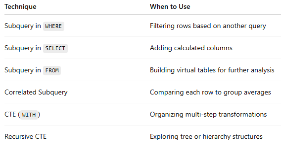
🧩 10 Practice Exercises

Try these on your own (I can give full runnable answers if you want next):

Create an employees table (name, dept, salary). Find employees earning above the average salary using a subquery.
Create a sales table. Show each category and its % of total revenue using a subquery in FROM.
Using a students and marks table, find students who scored above the class average.
Build a products table and use a correlated subquery to find products priced above their category’s average.
Create customers and orders tables. Use IN and EXISTS to find customers who placed orders.
Use a CTE to first compute total sales per region, then compute each region’s share of total sales.
Chain multiple CTEs: step 1 = purchases, step 2 = refunds, step 3 = net revenue.
Use a CTE to find top 3 customers by total spend.
Create a small organization table and write a recursive CTE to display the reporting hierarchy.
Create a CTE that filters out customers with zero orders, then use that result to find average spending among active customers.

Chapter 5 — Window Functions

(Plain-English guide + detailed examples with data + 10 exercises)

Welcome back, Bavi 👏 — this is one of the most powerful and useful SQL chapters, especially for AI, analytics, and time-series work.

Window functions let you perform calculations across rows — without grouping them together.
They are the secret behind rankings, running totals, moving averages, time-based comparisons, and feature engineering for machine learning models.

🧠 What You’ll Learn in This Chapter

By the end of this chapter, you’ll be able to:

Understand what window functions are and how they differ from normal aggregates.
Use OVER() and PARTITION BY.
Rank rows using ROW_NUMBER(), RANK(), and DENSE_RANK().
Compare current vs previous row using LAG() and LEAD().
Compute running totals and moving averages.
Use frame clauses like ROWS BETWEEN … for rolling calculations.

Every example below is fully runnable (it drops and creates its own tables).
You can copy each one directly into pgAdmin or DBeaver and it’ll just work ✅

💡 1. What Are Window Functions (In Simple Terms)

A window function looks at a “window” of rows — which can be:

all rows,
rows in the same group (partition),
or a subset around the current row (like “previous 2 and next 2”).

It does not collapse rows like GROUP BY does.
You still see every row, but you can add running totals, ranks, or differences as extra columns.

🔹 2. Basic Window Function Syntax

function_name(expression) OVER (
    PARTITION BY column
    ORDER BY column
    ROWS BETWEEN ... AND ...
)

Parts:

PARTITION BY: divide rows into groups (like GROUP BY but rows remain visible)
ORDER BY: defines order inside each group
ROWS BETWEEN: defines the window range

🧩 Example 1 — Compare Window vs Aggregate

-- EX1: Window vs Group Aggregate
DROP TABLE IF EXISTS ex1_sales;
CREATE TABLE ex1_sales (
  region TEXT,
  rep TEXT,
  sales NUMERIC(8,2)
);

INSERT INTO ex1_sales (region, rep, sales) VALUES
(’East’,’Alice’,100),
(’East’,’Bob’,150),
(’West’,’Cathy’,200),
(’West’,’Dan’,300),
(’West’,’Ella’,100);

-- Normal aggregate (collapses rows)
SELECT region, SUM(sales) AS total_sales
FROM ex1_sales
GROUP BY region;

-- Window aggregate (keeps all rows)
SELECT
  region,
  rep,
  sales,
  SUM(sales) OVER (PARTITION BY region) AS region_total
FROM ex1_sales
ORDER BY region, rep;

Plain Explanation:

The GROUP BY query loses individual reps — it only shows totals.
The OVER(PARTITION BY region) query keeps each rep and adds the total for their region beside them.

🧩 Example 2 — ROW_NUMBER(), RANK(), DENSE_RANK()

-- EX2: Ranking examples
DROP TABLE IF EXISTS ex2_scores;
CREATE TABLE ex2_scores (
  student TEXT,
  subject TEXT,
  marks INTEGER
);

INSERT INTO ex2_scores (student, subject, marks) VALUES
(’Anita’,’Math’,90),
(’Ben’,’Math’,85),
(’Carmen’,’Math’,85),
(’David’,’Math’,70),
(’Ella’,’Math’,95);

-- Ranking functions
SELECT
  student,
  subject,
  marks,
  ROW_NUMBER() OVER (PARTITION BY subject ORDER BY marks DESC) AS row_num,
  RANK() OVER (PARTITION BY subject ORDER BY marks DESC) AS rank_value,
  DENSE_RANK() OVER (PARTITION BY subject ORDER BY marks DESC) AS dense_rank_value
FROM ex2_scores
ORDER BY marks DESC;

Layman’s Explanation:

ROW_NUMBER() gives unique increasing numbers even for ties.
RANK() leaves gaps after ties (1, 2, 2, 4).
DENSE_RANK() doesn’t leave gaps (1, 2, 2, 3).
These are essential for leaderboards, ranking models, or finding top-N per category.

🧩 Example 3 — LAG() and LEAD() for Time-Series Comparison

-- EX3: LAG and LEAD
DROP TABLE IF EXISTS ex3_stock;
CREATE TABLE ex3_stock (
  stock_date DATE,
  symbol TEXT,
  price NUMERIC(8,2)
);

INSERT INTO ex3_stock (stock_date, symbol, price) VALUES
(’2025-01-01’,’AAPL’,100),
(’2025-01-02’,’AAPL’,105),
(’2025-01-03’,’AAPL’,102),
(’2025-01-04’,’AAPL’,110),
(’2025-01-05’,’AAPL’,108);

SELECT
  stock_date,
  symbol,
  price,
  LAG(price) OVER (PARTITION BY symbol ORDER BY stock_date) AS prev_price,
  LEAD(price) OVER (PARTITION BY symbol ORDER BY stock_date) AS next_price,
  price - LAG(price) OVER (PARTITION BY symbol ORDER BY stock_date) AS daily_change
FROM ex3_stock
ORDER BY stock_date;

Plain Explanation:

LAG() gives you the previous row’s value.
LEAD() gives the next row’s value.
You can calculate price - LAG(price) to find daily changes.
This is perfect for AI time-series features like “change from previous day”.

🧩 Example 4 — Running Total & Cumulative Sum

-- EX4: Running total per customer
DROP TABLE IF EXISTS ex4_orders;
CREATE TABLE ex4_orders (
  order_id SERIAL PRIMARY KEY,
  customer TEXT,
  order_date DATE,
  amount NUMERIC(8,2)
);

INSERT INTO ex4_orders (customer, order_date, amount) VALUES
(’Asha’,’2025-01-01’,100),
(’Asha’,’2025-01-03’,50),
(’Asha’,’2025-01-05’,150),
(’Ben’,’2025-01-02’,200),
(’Ben’,’2025-01-04’,100);

SELECT
  customer,
  order_date,
  amount,
  SUM(amount) OVER (PARTITION BY customer ORDER BY order_date) AS running_total
FROM ex4_orders
ORDER BY customer, order_date;

Explanation:
SUM(...) OVER (PARTITION BY customer ORDER BY order_date) keeps a running total as you move through time.
It doesn’t reset the rows — just adds a new column.

🧩 Example 5 — Moving Average (Rolling Window)

-- EX5: Moving average (3-day window)
DROP TABLE IF EXISTS ex5_temps;
CREATE TABLE ex5_temps (
  reading_date DATE,
  city TEXT,
  temp_c NUMERIC(5,2)
);

INSERT INTO ex5_temps (reading_date, city, temp_c) VALUES
(’2025-01-01’,’Paris’,10),
(’2025-01-02’,’Paris’,12),
(’2025-01-03’,’Paris’,14),
(’2025-01-04’,’Paris’,16),
(’2025-01-05’,’Paris’,18),
(’2025-01-06’,’Paris’,20);

SELECT
  reading_date,
  city,
  temp_c,
  ROUND(AVG(temp_c) OVER (
    PARTITION BY city
    ORDER BY reading_date
    ROWS BETWEEN 2 PRECEDING AND CURRENT ROW
  ),2) AS moving_avg_3days
FROM ex5_temps
ORDER BY reading_date;

Layman’s Explanation:
This keeps a moving average of the last 3 days (2 PRECEDING + current).
It’s essential for trend detection and smoothing in time-series analysis.

🧩 Example 6 — Percent Rank and Cumulative Distribution

-- EX6: Percent rank and cumulative distribution
DROP TABLE IF EXISTS ex6_scores;
CREATE TABLE ex6_scores (
  student TEXT,
  marks INTEGER
);

INSERT INTO ex6_scores (student, marks) VALUES
(’A’,90),(’B’,80),(’C’,70),(’D’,60),(’E’,50);

SELECT
  student,
  marks,
  PERCENT_RANK() OVER (ORDER BY marks) AS percent_rank,
  CUME_DIST() OVER (ORDER BY marks) AS cumulative_distribution
FROM ex6_scores
ORDER BY marks;

Plain Explanation:

PERCENT_RANK() gives rank as a percentage of total rows.
CUME_DIST() shows the proportion of rows less than or equal to current row.
These are great for normalizing scores or creating percentile-based features in ML.

🧩 Example 7 — Combine LAG + Window for Change Detection

-- EX7: Detect change events
DROP TABLE IF EXISTS ex7_device;
CREATE TABLE ex7_device (
  device_id TEXT,
  reading_ts TIMESTAMP,
  status TEXT
);

INSERT INTO ex7_device (device_id, reading_ts, status) VALUES
(’D1’,’2025-01-01 10:00’,’ON’),
(’D1’,’2025-01-01 11:00’,’ON’),
(’D1’,’2025-01-01 12:00’,’OFF’),
(’D1’,’2025-01-01 13:00’,’OFF’),
(’D1’,’2025-01-01 14:00’,’ON’);

SELECT
  device_id,
  reading_ts,
  status,
  LAG(status) OVER (PARTITION BY device_id ORDER BY reading_ts) AS prev_status,
  CASE WHEN status <> LAG(status) OVER (PARTITION BY device_id ORDER BY reading_ts)
       THEN ‘CHANGED’
       ELSE ‘SAME’
  END AS change_flag
FROM ex7_device
ORDER BY reading_ts;

Layman’s Explanation:
We compare the current status with the previous one using LAG().
This helps detect status changes, anomalies, or events — very common in IoT, logs, and monitoring datasets.

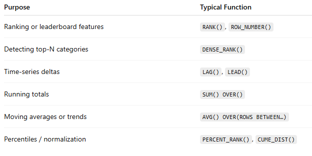
🧩 When to Use Window Functions in AI/ML

🧩 10 Practice Exercises

Try writing these queries in PostgreSQL. (I can give full runnable solutions if you want next.)

Create a sales(region, rep, sales_amount) table. Show each rep’s sales and total sales of their region using a window function.
Create students(name, score) and rank them using ROW_NUMBER(), RANK(), and DENSE_RANK().
Create orders(customer, order_date, amount) and compute each customer’s running total of spending.
Create a temperature(city, reading_date, temp) table and compute 7-day moving average temperature.
Using LAG(), find daily price changes for a stock(symbol, date, price) table.
Using LEAD(), predict next day’s value for each row in a time-series table.
Create scores(student, subject, marks) and find percentile ranks using PERCENT_RANK().
Using LAG(), detect when an IoT device changes its status (ON → OFF or OFF → ON).
Combine RANK() + PARTITION BY region to find top 2 sales reps per region.
Combine multiple window functions: for each customer, show total spent, running total, and percentage of total revenue.

Chapter 6 — Data Manipulation (INSERT · UPDATE · DELETE · MERGE · Transactions)

(Plain-English explanations + fully runnable SQL + 10 hands-on exercises)

🎯 Why this matters

Up to now you’ve learned how to read and analyze data.
This chapter teaches you how to change it safely: add new rows, fix mistakes, remove bad data, and merge new information — the day-to-day skills of any data engineer or AI-pipeline maintainer.

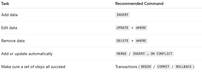
🧱 Core ideas in very simple words

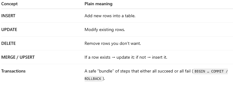
🧩 Example 1 — INSERT (single & multiple rows)

-- EX1: INSERT rows
DROP TABLE IF EXISTS ex1_products;
CREATE TABLE ex1_products (
  product_id SERIAL PRIMARY KEY,
  name TEXT,
  price NUMERIC(8,2),
  category TEXT
);

-- one row
INSERT INTO ex1_products (name, price, category)
VALUES (’Notebook’, 3.50, ‘Stationery’);

-- multiple rows
INSERT INTO ex1_products (name, price, category) VALUES
(’Pen’, 1.00, ‘Stationery’),
(’Espresso Beans’, 12.00, ‘Beverage’),
(’Green Tea’, 9.00, ‘Beverage’);

SELECT * FROM ex1_products;

Plain talk: INSERT adds new sheets to your filing cabinet. You can insert one or many rows in a single shot.

🧩 Example 2 — UPDATE (change existing data)

-- EX2: UPDATE
UPDATE ex1_products
SET price = price * 1.10
WHERE category = ‘Beverage’;  -- raise Beverage prices by 10%

-- give Pen a better name
UPDATE ex1_products
SET name = ‘Blue Pen’
WHERE name = ‘Pen’;

SELECT * FROM ex1_products;

What’s happening: SET tells PostgreSQL which columns to change. WHERE ensures you only change the right rows.
⚠ Without WHERE, you’d update every row.

🧩 Example 3 — DELETE (remove rows)

-- EX3: DELETE
DELETE FROM ex1_products
WHERE price < 2.00;  -- remove cheap items

SELECT * FROM ex1_products;

Tip: Always run a SELECT … WHERE … first to preview which rows will be deleted.

🧩 Example 4 — RETURNING clause

PostgreSQL can return changed rows immediately.

-- EX4: UPDATE … RETURNING
UPDATE ex1_products
SET price = price + 1.00
WHERE category = ‘Stationery’
RETURNING product_id, name, price;

Why useful: When your Python script updates data, RETURNING lets you grab new values without another query.

🧩 Example 5 — INSERT … RETURNING id

-- EX5: get new ID right after insert
INSERT INTO ex1_products (name, price, category)
VALUES (’Mug’, 6.00, ‘Merch’)
RETURNING product_id, name;

Perfect when you need to insert then use that new ID immediately in another table.

🧩 Example 6 — MERGE (UPSERT)

-- EX6: MERGE (PostgreSQL 15+)
DROP TABLE IF EXISTS ex6_inventory;
CREATE TABLE ex6_inventory (
  sku TEXT PRIMARY KEY,
  stock INT,
  price NUMERIC(8,2)
);

INSERT INTO ex6_inventory VALUES
(’A1’,10,5.00),
(’A2’,20,7.00);

-- new data to merge
DROP TABLE IF EXISTS ex6_updates;
CREATE TABLE ex6_updates (sku TEXT, stock INT, price NUMERIC(8,2));
INSERT INTO ex6_updates VALUES
(’A2’,25,7.50),  -- existing -> update
(’A3’,10,6.00);  -- new -> insert

MERGE INTO ex6_inventory AS inv
USING ex6_updates AS upd
ON inv.sku = upd.sku
WHEN MATCHED THEN
  UPDATE SET stock = upd.stock, price = upd.price
WHEN NOT MATCHED THEN
  INSERT (sku, stock, price) VALUES (upd.sku, upd.stock, upd.price);

SELECT * FROM ex6_inventory;

Plain explanation:
If the SKU already exists → update it.
If it’s new → insert it.
That’s an upsert — a combo of “update + insert”.

🧩 Example 7 — Transaction safety (BEGIN / COMMIT / ROLLBACK)

-- EX7: Transactions
BEGIN;

INSERT INTO ex1_products (name, price, category)
VALUES (’Temp Product’, 1.00, ‘Test’);

-- Oops! decide to cancel
ROLLBACK;

-- check: no “Temp Product” remains
SELECT * FROM ex1_products;

Layman’s view:
A transaction is like writing in pencil until you’re sure.
BEGIN starts the block.
COMMIT = keep changes.
ROLLBACK = erase everything since BEGIN.

🧩 Example 8 — COMMIT success path

BEGIN;
UPDATE ex1_products SET price = price + 0.5 WHERE category=’Merch’;
COMMIT;

Now the price bump stays permanently.

🧩 Example 9 — Bulk INSERT using COPY (simulated)

-- EX9: COPY for bulk load (works in psql or pgAdmin)
-- COPY ex1_products(name,price,category)
-- FROM ‘/path/to/file.csv’
-- DELIMITER ‘,’ CSV HEADER;

Plain note: For large AI datasets you’ll load CSVs quickly using COPY; it’s faster than millions of INSERTs.

🧩 Example 10 — DELETE with JOIN (subquery style)

-- EX10: Delete discontinued items using subquery
DROP TABLE IF EXISTS ex10_products;
DROP TABLE IF EXISTS ex10_discontinued;

CREATE TABLE ex10_products (id SERIAL PRIMARY KEY, name TEXT);
CREATE TABLE ex10_discontinued (name TEXT);

INSERT INTO ex10_products (name) VALUES
(’Pen’),(’Pencil’),(’Notebook’),(’Marker’);

INSERT INTO ex10_discontinued (name) VALUES
(’Pencil’),(’Marker’);

DELETE FROM ex10_products
WHERE name IN (SELECT name FROM ex10_discontinued);

SELECT * FROM ex10_products;

Why: Sometimes deletions depend on another table — subqueries make it easy.

⚙️ Quick real-world hints

🧩 10 Practice Exercises

Create a users table and insert 5 rows. Update one user’s email, then delete another.
Insert 10 rows into a books table in a single INSERT statement.
Build an inventory(sku, stock) table; write a MERGE that updates stock if SKU exists else inserts it.
Create orders(order_id, amount) and refunds(order_id, amount); use a transaction to deduct refunds safely.
Simulate a mistake: begin a transaction, delete all rows, then ROLLBACK — verify restoration.
Use RETURNING to get the IDs of newly added products.
Create customers and addresses; insert a customer, then insert address using the returned ID.
Create a students table and bulk-insert sample data (5 rows at once).
Write an UPDATE that increases all salaries in the employees table by 5 %.
Using DELETE … WHERE id IN (SELECT …), remove inactive users listed in another table.

Chapter 7 — Data Cleaning & Transformation

(Plain-English + fully runnable PostgreSQL examples + 10 exercises)

🎯 Why this matters

In real AI and data science work, raw data is always messy.
Before it can be used for analysis or model training, you need to clean, standardize, and transform it — fixing spaces, inconsistent cases, dates, duplicates, missing values, and bad formats.

In PostgreSQL, this is easy once you know string functions, date/time functions, type conversions, and even pivot/unpivot operations.

This chapter shows you exactly how to clean and shape data so your AI scripts or Power BI dashboards work flawlessly.

🧠 What You’ll Learn

Clean text fields (trim, lower, replace, split)
Work with dates and times (extract parts, add/subtract days)
Convert data types safely
Handle NULLs and default values
Pivot/unpivot data for analytics
Use conditional transforms (CASE WHEN)

Each example is fully copy-paste runnable — each creates its own small tables.

🧩 Example 1 — Trimming, Upper/Lower Case, Replacing

-- EX1: String cleaning basics
DROP TABLE IF EXISTS ex1_customers;
CREATE TABLE ex1_customers (
  id SERIAL PRIMARY KEY,
  raw_name TEXT,
  raw_email TEXT
);

INSERT INTO ex1_customers (raw_name, raw_email) VALUES
(’   anita  ‘, ‘Anita@Example.COM  ‘),
(’BEN’, ‘ben@example.com’),
(’ cArMen ‘, ‘CARMEN@EXAMPLE.COM’);

SELECT
  id,
  raw_name,
  TRIM(raw_name) AS name_trimmed,
  INITCAP(TRIM(raw_name)) AS name_clean,      -- Capitalize first letter
  LOWER(TRIM(raw_email)) AS email_clean       -- lowercase all
FROM ex1_customers;

Plain Explanation:

TRIM() removes unwanted spaces.
INITCAP() makes “cArMen” → “Carmen”.
LOWER() fixes inconsistent email cases.
Combining these gives uniform data — perfect for ML preprocessing or joins.

🧩 Example 2 — REPLACE, SUBSTRING, CONCAT, and String Splitting

-- EX2: Replace and extract text
DROP TABLE IF EXISTS ex2_products;
CREATE TABLE ex2_products (
  raw_code TEXT
);

INSERT INTO ex2_products VALUES
(’ SKU-123-RED ‘),
(’SKU-456-BLUE’),
(’ sku-789-green ‘);

SELECT
  TRIM(UPPER(raw_code)) AS code_clean,
  REPLACE(TRIM(UPPER(raw_code)),’SKU-’,’‘) AS code_no_prefix,
  SUBSTRING(raw_code FROM 5 FOR 3) AS part_extract,
  CONCAT(’Product:’, TRIM(raw_code)) AS label,
  SPLIT_PART(TRIM(UPPER(raw_code)),’-’,3) AS color
FROM ex2_products;

Plain Explanation:

REPLACE() deletes unwanted text.
SUBSTRING() extracts part of a string.
CONCAT() glues text together.
SPLIT_PART() extracts parts separated by a character (like color in code).

🧩 Example 3 — Handling NULLs: COALESCE & NULLIF

-- EX3: COALESCE and NULLIF
DROP TABLE IF EXISTS ex3_payments;
CREATE TABLE ex3_payments (
  id SERIAL PRIMARY KEY,
  card_number TEXT,
  backup_card TEXT
);

INSERT INTO ex3_payments (card_number, backup_card) VALUES
(NULL, ‘1234-XXXX’),
(’9876-YYYY’, NULL),
(NULL, NULL);

SELECT
  id,
  card_number,
  backup_card,
  COALESCE(card_number, backup_card, ‘NO CARD’) AS chosen_card
FROM ex3_payments;

Plain Explanation:

COALESCE() returns the first non-NULL value.
(If both are NULL → “NO CARD”).
NULLIF(a,b) returns NULL if a=b, useful for removing dummy values like “N/A”.

🧩 Example 4 — Date Cleaning & Extracting

-- EX4: Working with dates
DROP TABLE IF EXISTS ex4_orders;
CREATE TABLE ex4_orders (
  order_id SERIAL PRIMARY KEY,
  raw_date TEXT
);

INSERT INTO ex4_orders (raw_date) VALUES
(’2025-03-05’),
(’ 2025/03/06 ‘),
(’March 07 2025’);

SELECT
  order_id,
  raw_date,
  TO_DATE(TRIM(raw_date),’YYYY-MM-DD’) AS fmt_1,
  TO_DATE(TRIM(raw_date),’YYYY/MM/DD’) AS fmt_2,
  TO_DATE(TRIM(raw_date),’Month DD YYYY’) AS fmt_3
FROM ex4_orders;

-- Use EXTRACT to get date parts
SELECT
  CURRENT_DATE AS today,
  EXTRACT(YEAR FROM CURRENT_DATE) AS this_year,
  EXTRACT(MONTH FROM CURRENT_DATE) AS month_no,
  EXTRACT(DAY FROM CURRENT_DATE) AS day_no;

Plain Explanation:

TO_DATE(text, format) converts strings into real dates.
EXTRACT() pulls out parts like year/month/day for grouping or trend analysis.

🧩 Example 5 — DATE Arithmetic (Add/Subtract days)

-- EX5: Date math
SELECT
  CURRENT_DATE AS today,
  CURRENT_DATE + INTERVAL ‘7 days’ AS plus_7days,
  CURRENT_DATE - INTERVAL ‘1 month’ AS last_month,
  AGE(CURRENT_DATE, DATE ‘2024-12-31’) AS diff_age;

Why important: For time-based AI features like “days since signup” or “tenure before churn”.

🧩 Example 6 — Type Conversion (CAST and ::)

-- EX6: Type conversions
DROP TABLE IF EXISTS ex6_conversion;
CREATE TABLE ex6_conversion (
  txt_num TEXT
);

INSERT INTO ex6_conversion VALUES (’100’), (’250.75’), (’NaN’);

SELECT
  txt_num,
  CAST(txt_num AS NUMERIC) AS num_value,
  txt_num::NUMERIC AS short_cast
FROM ex6_conversion
WHERE txt_num ~ ‘^[0-9.]+$’; -- regex to keep numeric-looking rows

Plain Explanation:
CAST() or :: changes data type — text to number, date to text, etc.
We used regex (~ ‘^[0-9.]+$’) to ignore “NaN”.

🧩 Example 7 — Conditional Transformation with CASE WHEN

-- EX7: CASE WHEN cleaning
DROP TABLE IF EXISTS ex7_feedback;
CREATE TABLE ex7_feedback (
  rating INTEGER
);

INSERT INTO ex7_feedback VALUES (5),(4),(3),(2),(1),(NULL);

SELECT
  rating,
  CASE
    WHEN rating >= 4 THEN ‘Positive’
    WHEN rating = 3 THEN ‘Neutral’
    WHEN rating < 3 THEN ‘Negative’
    ELSE ‘No Rating’
  END AS sentiment
FROM ex7_feedback;

Plain Explanation:
CASE WHEN gives logic inside SQL — like if-elif-else in Python.

🧩 Example 8 — Pivoting data (rows → columns)

-- EX8: Pivot data using crosstab()
CREATE EXTENSION IF NOT EXISTS tablefunc;

DROP TABLE IF EXISTS ex8_sales;
CREATE TABLE ex8_sales (
  region TEXT,
  month TEXT,
  amount NUMERIC(8,2)
);

INSERT INTO ex8_sales VALUES
(’East’,’Jan’,100),(’East’,’Feb’,120),(’West’,’Jan’,150),(’West’,’Feb’,130);

SELECT * FROM crosstab(
  ‘SELECT region, month, amount FROM ex8_sales ORDER BY 1,2’,
  $$VALUES (’Jan’), (’Feb’)$$
) AS ct(region TEXT, Jan NUMERIC, Feb NUMERIC);

Plain Explanation:
crosstab() rotates rows into columns.
Used for quick summaries — like Excel pivot tables.

🧩 Example 9 — Unpivoting data (columns → rows)

-- EX9: Unpivot with UNION ALL
DROP TABLE IF EXISTS ex9_quarter_sales;
CREATE TABLE ex9_quarter_sales (
  region TEXT,
  q1 NUMERIC,
  q2 NUMERIC
);

INSERT INTO ex9_quarter_sales VALUES (’East’,100,200), (’West’,150,180);

SELECT region, ‘Q1’ AS quarter, q1 AS sales FROM ex9_quarter_sales
UNION ALL
SELECT region, ‘Q2’, q2 FROM ex9_quarter_sales;

Plain Explanation:
UNION ALL stacks columns vertically to normalize data — great for analytics pipelines.

🧩 Example 10 — Combining multiple cleaning operations

-- EX10: All-in-one cleaning
DROP TABLE IF EXISTS ex10_raw_users;
CREATE TABLE ex10_raw_users (
  id SERIAL,
  full_name TEXT,
  join_date TEXT,
  country TEXT
);

INSERT INTO ex10_raw_users (full_name, join_date, country) VALUES
(’  alice smith ‘, ‘2025/01/05 ‘, ‘usa’),
(’BEN ‘, ‘05-01-2025’, ‘Uk ‘),
(’  carmen de souza’, ‘2025-01-07’, ‘ INDIA’);

SELECT
  id,
  INITCAP(TRIM(full_name)) AS clean_name,
  TO_DATE(TRIM(join_date), ‘YYYY/MM/DD’) 
     FILTER (WHERE join_date LIKE ‘2025/%’) 
     AS join_date1,
  COALESCE(TO_DATE(TRIM(join_date), ‘DD-MM-YYYY’),
           TO_DATE(TRIM(join_date), ‘YYYY-MM-DD’)) AS join_date_fixed,
  UPPER(TRIM(country)) AS country_clean
FROM ex10_raw_users;

Explanation:
We combined trimming, case fixing, date parsing, and null-safe conversions — exactly what real-world cleaning looks like before AI preprocessing.

🧩 10 Practice Exercises

Try these in PostgreSQL:

Create a users table with messy names and emails; use TRIM, INITCAP, and LOWER to clean them.
Use REPLACE to remove “SKU-” prefix from product codes and SPLIT_PART to extract the color name.
Use COALESCE to fill NULL phone numbers with a default “Not Provided”.
Convert a text date column ‘2025/03/10’ to a real DATE type using TO_DATE.
Extract YEAR and MONTH from a timestamp column using EXTRACT().
Add 30 days to all subscription start dates using INTERVAL ‘30 days’.
Use CASE WHEN to classify ratings into “Good”, “Average”, “Poor”.
Pivot a small table with sales by month into columns using crosstab().
Unpivot quarterly columns into rows using UNION ALL.
Create a combined cleaning query that trims spaces, fixes case, and converts a join_date to DATE type.

Chapter 8 — JSON, Arrays & Advanced Data Types in PostgreSQL

(Plain-English + fully runnable examples + 10 practice exercises)

🎯 Why this matters

In modern AI, ML, and analytics projects, data often comes in semi-structured formats — JSON from APIs, logs from IoT devices, lists of tags or labels, etc.
PostgreSQL shines here because it natively understands JSON, arrays, and key-value data — letting you store, query, and transform complex data without extra tools.

This chapter will show you how to use these features cleanly and safely.

🧠 What You’ll Learn

What JSON and JSONB are, and when to use them
How to insert, query, and update JSON values
Access nested JSON keys with → and →>
Use JSON functions (jsonb_each, jsonb_array_elements, etc.)
Store and search arrays (ARRAY[], unnest())
Use range and enum types for clean data modelling

Every example below is copy-paste runnable and self-contained.

🧩 Example 1 — Storing and Retrieving JSON

-- EX1: JSON basics
DROP TABLE IF EXISTS ex1_profiles;
CREATE TABLE ex1_profiles (
  id SERIAL PRIMARY KEY,
  user_info JSONB
);

INSERT INTO ex1_profiles (user_info) VALUES
(’{”name”: “Alice”, “age”: 28, “skills”: [”Python”, “SQL”, “ML”]}’),
(’{”name”: “Ben”, “age”: 35, “skills”: [”Java”, “DevOps”]}’);

-- select entire JSON
SELECT user_info FROM ex1_profiles;

-- extract individual keys
SELECT
  user_info->>’name’ AS name,
  user_info->>’age’  AS age,
  user_info->’skills’ AS skills_array
FROM ex1_profiles;

Layman’s explanation:

-> gives a JSON object or array.
->> gives plain text.
JSONB stores JSON in a binary format for faster search.

🧩 Example 2 — Filtering JSON fields

-- EX2: filter by JSON key
SELECT *
FROM ex1_profiles
WHERE (user_info->>’age’)::INT > 30;

Explanation: cast the extracted text to integer and filter — same as any normal column.

🧩 Example 3 — Querying inside JSON arrays

-- EX3: search within skills array
SELECT
  user_info->>’name’ AS name,
  user_info->’skills’ AS skills
FROM ex1_profiles
WHERE user_info->’skills’ @> ‘[”SQL”]’::jsonb;

Explanation:
@> means “contains”.
So skills @> [”SQL”] finds anyone whose skills include SQL.

🧩 Example 4 — Expanding JSON arrays to rows

-- EX4: jsonb_array_elements()
SELECT
  user_info->>’name’ AS name,
  skill.value AS each_skill
FROM ex1_profiles,
     jsonb_array_elements(user_info->’skills’) AS skill;

Plain talk:
jsonb_array_elements() unpacks an array so you can treat each element as a row — perfect for normalizing JSON data.

🧩 Example 5 — Updating JSON fields

-- EX5: update a key inside JSON
UPDATE ex1_profiles
SET user_info = jsonb_set(user_info, ‘{city}’, ‘”Brussels”’)
WHERE user_info->>’name’ = ‘Alice’;

SELECT user_info FROM ex1_profiles;

Explanation:
jsonb_set(target, path, new_value) inserts or replaces a value at a JSON path.
‘{city}’ means top-level key “city”.

🧩 Example 6 — Nested JSON structure

-- EX6: nested JSON example
DROP TABLE IF EXISTS ex6_orders;
CREATE TABLE ex6_orders (data JSONB);

INSERT INTO ex6_orders VALUES
(’{
   “order_id”:101,
   “customer”:{”name”:”Asha”,”city”:”Paris”},
   “items”:[{”product”:”Pen”,”qty”:3},{”product”:”Notebook”,”qty”:2}]
 }’);

-- access nested keys
SELECT
  data->’customer’->>’name’ AS customer_name,
  data->’items’->0->>’product’ AS first_product
FROM ex6_orders;

Plain Explanation:
Use chained -> and ->> to drill down into nested levels.

🧩 Example 7 — JSON aggregation

-- EX7: aggregate to JSON
DROP TABLE IF EXISTS ex7_books;
CREATE TABLE ex7_books (author TEXT, title TEXT);

INSERT INTO ex7_books VALUES
(’Alice’,’Postgres Made Easy’),
(’Alice’,’Python for Data’),
(’Ben’,’DevOps 101’);

SELECT author, jsonb_agg(title) AS books
FROM ex7_books
GROUP BY author;

Explanation:
jsonb_agg() gathers rows into a JSON array — very handy for building API responses.

🧩 Example 8 — Arrays in PostgreSQL

-- EX8: array basics
DROP TABLE IF EXISTS ex8_students;
CREATE TABLE ex8_students (
  name TEXT,
  scores INT[]
);

INSERT INTO ex8_students VALUES
(’Anita’, ARRAY[85,90,95]),
(’Ben’, ARRAY[70,75,80]);

SELECT
  name,
  scores,
  scores[1] AS first_exam,
  unnest(scores) AS each_score
FROM ex8_students;

Plain Explanation:

Arrays are declared as type[].
Use [n] to access an element.
unnest() turns array elements into rows.

🧩 Example 9 — Searching arrays

-- EX9: find students who scored 90
SELECT name, scores
FROM ex8_students
WHERE 90 = ANY(scores);

-- who has all scores > 80
SELECT name
FROM ex8_students
WHERE NOT EXISTS (
  SELECT 1 FROM unnest(scores) s WHERE s < 80
);

Explanation:
ANY() checks if a value is in the array.
You can also unnest to run more complex conditions.

🧩 Example 10 — Range and Enum types

-- EX10: ranges and enums
DROP TABLE IF EXISTS ex10_tasks;
CREATE TYPE task_status AS ENUM (’todo’,’in_progress’,’done’);

CREATE TABLE ex10_tasks (
  id SERIAL,
  title TEXT,
  status task_status,
  active_period DATERANGE
);

INSERT INTO ex10_tasks (title,status,active_period) VALUES
(’Build API’,’in_progress’,’[2025-01-01,2025-01-10)’),
(’Write Docs’,’todo’,’[2025-02-01,2025-02-05)’);

SELECT
  title,
  status,
  LOWER(active_period) AS start_date,
  UPPER(active_period) AS end_date,
  UPPER(active_period) - LOWER(active_period) AS days_span
FROM ex10_tasks;

Plain Explanation:

ENUM keeps only predefined values (great for data consistency).
DATERANGE stores a start-to-end range.
LOWER() and UPPER() pull the endpoints.

🧩 10 Practice Exercises

Try these yourself:

Create a profiles table with a JSONB column and store name, age, and city. Extract only names where city=’Paris’.
From a JSON column containing arrays of skills, unnest all skills into separate rows.
Update a JSONB object by adding a new key “country”: “Belgium”.
Create a nested JSON of orders and access the second item’s product name.
Use jsonb_agg() to group employee names by department.
Build a students(name, grades int[]) table and find who has any score below 60.
Use unnest() to list all scores for each student.
Create an ENUM type mood (’happy’,’neutral’,’sad’) and insert sample data.
Create a daterange column for a project timeline; show duration using UPPER() - LOWER().
Combine JSON and array: store user profile JSON with a list of preferred languages and query users who include ‘Python’.

Chapter 9 — Performance & Optimization

(Simple explanations + runnable SQL demos + 10 practice exercises)

🎯 Why this chapter matters

When your tables grow from a few hundred rows to millions, even correct SQL can crawl.
Learning a handful of tuning tricks—indexes, query plans, and query-writing habits—makes the difference between a 5-second and a 5-millisecond result.

🧠 What You’ll Learn

How PostgreSQL looks for data (execution plans)
How and when to create indexes
Primary vs secondary indexes
Reading EXPLAIN output
Reducing work with selective WHERE clauses and LIMIT
Using materialized views for expensive reports
Avoiding common slow-query mistakes

Every block below is safe to copy-paste—it drops and rebuilds its own tables.

🧩 Example 1 — Why indexes exist

-- EX1: full table scan
DROP TABLE IF EXISTS ex1_users;
CREATE TABLE ex1_users(id SERIAL PRIMARY KEY, name TEXT, city TEXT);
INSERT INTO ex1_users(name, city)
SELECT ‘User’||g, CASE WHEN g%3=0 THEN ‘Brussels’
                       WHEN g%3=1 THEN ‘London’
                       ELSE ‘Paris’ END
FROM generate_series(1,50000) g;

-- Without index
EXPLAIN ANALYZE SELECT * FROM ex1_users WHERE city=’Paris’;

-- Add index and rerun
CREATE INDEX idx_city ON ex1_users(city);
EXPLAIN ANALYZE SELECT * FROM ex1_users WHERE city=’Paris’;

Layman:
Before the index, PostgreSQL had to read every page—like flipping every sheet in a filing cabinet.
After the index, it jumps straight to the “Paris” pages.

🧩 Example 2 — Understanding `EXPLAIN`

EXPLAIN SELECT * FROM ex1_users WHERE city=’Paris’;
EXPLAIN ANALYZE SELECT * FROM ex1_users WHERE city=’Paris’;

Plain English:

EXPLAIN = show plan (what Postgres will do).
EXPLAIN ANALYZE = run it + show actual time.
Look for:

Seq Scan → sequential scan = no index used.
Index Scan → index used ✅.
Rows removed by filter → how many were checked but discarded.

🧩 Example 3 — Composite (index on multiple columns)

DROP INDEX IF EXISTS idx_city;
CREATE INDEX idx_city_name ON ex1_users(city, name);
EXPLAIN ANALYZE SELECT * FROM ex1_users
WHERE city=’Paris’ AND name LIKE ‘User1%’;

Tip: put the more selective column (city) first; Postgres filters it first.

🧩 Example 4 — Unique and Partial Indexes

-- unique index automatically created by PRIMARY KEY
-- partial index example: only London users
CREATE INDEX idx_london_only ON ex1_users(name)
WHERE city=’London’;

EXPLAIN ANALYZE SELECT * FROM ex1_users
WHERE city=’London’ AND name LIKE ‘User2%’;

Partial indexes speed up queries that always include a specific condition.

🧩 Example 5 — Avoid functions on indexed columns

-- Bad: function disables index
EXPLAIN SELECT * FROM ex1_users WHERE LOWER(city)=’paris’;

-- Good: store lowercase in another column or use expression index
CREATE INDEX idx_lower_city ON ex1_users((LOWER(city)));
EXPLAIN SELECT * FROM ex1_users WHERE LOWER(city)=’paris’;

Rule: if you wrap the column in a function, create a matching expression index.

🧩 Example 6 — Materialized Views (caching heavy queries)

-- EX6: cache total users per city
DROP MATERIALIZED VIEW IF EXISTS mv_city_counts;
CREATE MATERIALIZED VIEW mv_city_counts AS
SELECT city, COUNT(*) AS total
FROM ex1_users GROUP BY city;

SELECT * FROM mv_city_counts;

-- refresh when data changes
REFRESH MATERIALIZED VIEW mv_city_counts;

Think of materialized views as stored snapshots—faster for dashboards.

🧩 Example 7 — Limit and Pagination

EXPLAIN ANALYZE SELECT * FROM ex1_users ORDER BY id LIMIT 10 OFFSET 100;

LIMIT reduces work; combine with indexes on ORDER BY columns for speed.

🧩 Example 8 — Using `VACUUM ANALYZE`

VACUUM ANALYZE ex1_users;

Tells PostgreSQL to clean old rows and refresh statistics so the planner picks good indexes.

🧩 Example 9 — Rewriting for performance

-- slow
SELECT * FROM ex1_users WHERE city IN (SELECT city FROM ex1_users WHERE id<10);

-- faster equivalent using join
SELECT u.* FROM ex1_users u
JOIN (SELECT DISTINCT city FROM ex1_users WHERE id<10) c USING(city);

Joins are often faster than IN when subquery returns many rows.

🧩 Example 10 — EXPLAIN buffers and I/O timing

EXPLAIN (ANALYZE, BUFFERS) SELECT * FROM ex1_users WHERE city=’Paris’;

Shows memory/disk reads; use it to catch “I/O bound” queries.

⚙️ Quick Tuning Checklist

✅ Create indexes for columns used often in WHERE, JOIN, ORDER BY.
✅ Avoid wildcards at the start of LIKE ‘%term’.
✅ Use the smallest data type possible (INT vs BIGINT).
✅ Run ANALYZE after large changes.
✅ Batch inserts; avoid one row per transaction.
✅ Cache expensive aggregates in materialized views.

🧩 10 Practice Exercises

Build a customers(city, country) table with 100 K rows and test query speed with and without an index.
Create a composite index on (country, city) and compare EXPLAIN plans.
Write a query that benefits from a partial index (WHERE active=true).
Add an expression index on LOWER(email) and verify its use.
Use EXPLAIN ANALYZE to compare IN vs JOIN performance.
Create a materialized view summarizing total sales per month and refresh it.
Demonstrate a transaction with many inserts followed by one COMMIT; compare to per-row commits.
Delete 10 000 rows, run VACUUM ANALYZE, and note the difference in plan cost.
Show how LIMIT 10 changes query time compared to full scan.
Turn a slow correlated subquery into a join and confirm via EXPLAIN that the plan improves.

Chapter 10 — AI / Data-Specific SQL Use Cases

(Feature Engineering · Time Series · ETL Data Quality · Integration with Python)

🎯 Why this chapter matters

Everything you learned so far becomes truly powerful when you apply it to AI & ML data preparation.
In real projects, 70–80 % of the work before model training is SQL-based data wrangling—joining multiple data sources, engineering features, detecting anomalies, and validating ETL pipelines.

This chapter shows exactly how those techniques appear in production pipelines.

🧠 What You’ll Learn

Write SQL for feature engineering (ratios, lags, aggregates).
Do time-series transformations directly in PostgreSQL.
Build ETL data-quality checks with SQL.
Detect anomalies or missing values.
Combine SQL + Python for real-world model input pipelines.

All examples are copy-paste runnable.

🧩 Example 1 — Feature Engineering: ratios & counts

-- EX1: User activity features
DROP TABLE IF EXISTS ex1_activity;
CREATE TABLE ex1_activity(
  user_id INT, sessions INT, purchases INT, revenue NUMERIC(8,2)
);
INSERT INTO ex1_activity VALUES
(1,10,2,200),(2,15,5,500),(3,8,0,0),(4,20,10,900);

SELECT
  user_id,
  sessions,
  purchases,
  revenue,
  ROUND(revenue/purchases,2) AS avg_order_value,
  ROUND(purchases::NUMERIC/sessions,2) AS conversion_rate
FROM ex1_activity;

Idea: Create derived columns that describe behavior—these become model features.

🧩 Example 2 — Time-Series: rolling metrics

-- EX2: rolling 7-day sales
DROP TABLE IF EXISTS ex2_sales;
CREATE TABLE ex2_sales(day DATE, revenue NUMERIC);
INSERT INTO ex2_sales
SELECT d::DATE, (100 + random()*50)::INT
FROM generate_series(’2025-01-01’,’2025-01-20’,’1 day’) d;

SELECT
  day,
  revenue,
  ROUND(AVG(revenue) OVER(
      ORDER BY day ROWS BETWEEN 6 PRECEDING AND CURRENT ROW),2) AS avg_7d,
  SUM(revenue)  OVER(
      ORDER BY day ROWS BETWEEN 6 PRECEDING AND CURRENT ROW) AS sum_7d
FROM ex2_sales
ORDER BY day;

Why: Rolling windows capture short-term trends for forecasting.

🧩 Example 3 — Feature Lag for Prediction

-- EX3: previous-day revenue
SELECT
  day,
  revenue,
  LAG(revenue) OVER(ORDER BY day) AS prev_day,
  revenue - LAG(revenue) OVER(ORDER BY day) AS diff
FROM ex2_sales
ORDER BY day;

Use: previous-value deltas often feed time-series regression models.

🧩 Example 4 — Outlier & Anomaly Detection

-- EX4: find abnormal sales
WITH stats AS (
  SELECT AVG(revenue) AS mean, STDDEV_POP(revenue) AS sd FROM ex2_sales
)
SELECT s.day, s.revenue,
       CASE WHEN s.revenue > mean+2*sd THEN ‘High Outlier’
            WHEN s.revenue < mean-2*sd THEN ‘Low Outlier’
            ELSE ‘Normal’ END AS flag
FROM ex2_sales s, stats;

Layman: anything > 2 σ from mean is flagged—quick anomaly check before training.

🧩 Example 5 — Data Quality / ETL Checks

-- EX5: data-validation example
DROP TABLE IF EXISTS ex5_orders;
CREATE TABLE ex5_orders(id INT, amount NUMERIC, customer_id INT, order_date DATE);
INSERT INTO ex5_orders VALUES
(1,100,10,’2025-01-05’),
(2,NULL,11,’2025-01-06’),
(3,120,10,NULL),
(4,90,NULL,’2025-01-07’);

SELECT
  COUNT(*) FILTER(WHERE amount IS NULL)     AS missing_amount,
  COUNT(*) FILTER(WHERE customer_id IS NULL)AS missing_customer,
  COUNT(*) FILTER(WHERE order_date IS NULL) AS missing_date,
  COUNT(DISTINCT id)                        AS unique_ids
FROM ex5_orders;

Why: ETL jobs run these checks daily to prevent dirty data from entering AI pipelines.

🧩 Example 6 — Deduplication

-- EX6: remove duplicates keeping latest
DROP TABLE IF EXISTS ex6_logs;
CREATE TABLE ex6_logs(user_id INT, event_ts TIMESTAMP, source TEXT);
INSERT INTO ex6_logs VALUES
(1,’2025-01-01 10:00’,’web’),
(1,’2025-01-01 12:00’,’mobile’),
(1,’2025-01-01 12:00’,’mobile’); -- duplicate

DELETE FROM ex6_logs a
USING ex6_logs b
WHERE a.ctid<b.ctid AND a.user_id=b.user_id AND a.event_ts=b.event_ts;

SELECT * FROM ex6_logs;

Idea: Keep one row per unique key.

🧩 Example 7 — Creating Train/Test Splits

-- EX7: random split
DROP TABLE IF EXISTS ex7_dataset;
CREATE TABLE ex7_dataset(id SERIAL, feature NUMERIC);
INSERT INTO ex7_dataset(feature)
SELECT random()*100 FROM generate_series(1,20);

SELECT id, feature,
       CASE WHEN random()<0.8 THEN ‘train’ ELSE ‘test’ END AS dataset_split
FROM ex7_dataset;

Use: simple SQL-based splitting before exporting to Python.

🧩 Example 8 — Feature Scaling and Normalization

-- EX8: z-score normalization
SELECT
  feature,
  ROUND((feature - AVG(feature) OVER()) /
        STDDEV_POP(feature) OVER(),2) AS z_score
FROM ex7_dataset;

Why: scaled features help many ML models converge faster.

🧩 Example 9 — Combine SQL + Python (pandas integration)

# Python snippet (run separately)
import pandas as pd, sqlalchemy as sa
engine = sa.create_engine(”postgresql://user:pwd@localhost/db”)

df = pd.read_sql(”“”
    SELECT id, feature,
           (feature - AVG(feature) OVER()) / STDDEV_POP(feature) OVER() AS z
    FROM ex7_dataset
“”“, engine)

print(df.head())

Takeaway: use SQL for heavy lifting, pandas for downstream modeling.

🧩 Example 10 — Time-based Feature Store

-- EX10: daily aggregates ready for ML
WITH daily AS (
  SELECT DATE(event_ts) AS day, user_id, COUNT(*) AS actions
  FROM ex6_logs
  GROUP BY 1,2
),
user_stats AS (
  SELECT user_id,
         AVG(actions) AS avg_actions,
         MAX(actions) AS max_actions
  FROM daily GROUP BY user_id
)
SELECT * FROM user_stats;

Purpose: store compact per-user summaries for model input.

⚙️ Quick Checklist for AI Data in SQL

✅ Use window functions for temporal features.
✅ Normalize or bucket numeric columns.
✅ Run quality checks (COUNT NULL, outliers) before export.
✅ Use CTEs to chain transformations cleanly.
✅ Push as much aggregation logic as possible into PostgreSQL before moving data to Python.

🧩 10 Practice Exercises

Create a transactions table and build features: total_spend, avg_spend, transactions_last_7d.
Compute daily revenue change % using LAG().
Detect outliers beyond 3 × standard deviation.
Count missing fields per column for a dataset.
Write a deduplication query keeping the newest timestamp.
Generate a random 80/20 train-test split.
Standardize a numeric feature with z-score formula in SQL.
Create aggregated features per customer for ML (avg_order, max_order).
Build a materialized view that stores yesterday’s metrics for quick access.
Export aggregated data to Python (pandas) for model training.

Chapter 11 — Python Integration & Automation

(PostgreSQL + Python with pandas, SQLAlchemy, psycopg2 — ETL scripting, automation, and data pipelines)

🎯 Why this chapter matters

In real-world AI, ML, or data-engineering jobs, you rarely work inside the SQL shell.
You use Python as the controller — to run queries, fetch data, clean it, transform it further, and load it into models or dashboards.

This chapter connects everything you’ve learned in SQL to Python — turning PostgreSQL into a powerful backend for data pipelines, ETL jobs, and feature engineering systems.

🧠 What You’ll Learn

How to connect Python to PostgreSQL
Run queries and fetch results into pandas
Write data back to the database
Automate ETL scripts (Extract–Transform–Load)
Parameterize queries
Handle transactions safely in Python
Schedule recurring jobs

🧩 Example 1 — Connecting Python to PostgreSQL (SQLAlchemy + pandas)

# EX1: Basic connection and read
import pandas as pd
from sqlalchemy import create_engine

# connection string format:
# postgresql://username:password@host:port/database
engine = create_engine(”postgresql://postgres:password@localhost:5432/ai_course”)

# read data directly into pandas
df = pd.read_sql(”SELECT * FROM ex1_users LIMIT 5;”, engine)
print(df.head())

Plain Explanation:

SQLAlchemy builds the connection engine.
pd.read_sql() executes SQL and returns a DataFrame.
You can now use pandas functions like .describe() or .plot() on SQL data.

🧩 Example 2 — Writing Data from pandas to PostgreSQL

# EX2: Write dataframe to SQL
data = {
    “user_id”: [1, 2, 3],
    “score”: [85, 92, 76],
    “subject”: [”Math”, “AI”, “Data Science”]
}
df_new = pd.DataFrame(data)

df_new.to_sql(”student_scores”, engine, if_exists=”replace”, index=False)

print(”✅ Data written to PostgreSQL successfully!”)

Explanation:

if_exists=”replace” overwrites the table (use “append” to add).
pandas handles type conversion automatically.

🧩 Example 3 — Parameterized Query (Safe Against SQL Injection)

# EX3: parameterized query
import pandas as pd
from sqlalchemy import text

query = text(”SELECT * FROM ex1_users WHERE city = :city_name LIMIT 5”)
df_paris = pd.read_sql(query, engine, params={”city_name”: “Paris”})
print(df_paris)

Why this matters:
Using placeholders (:city_name) avoids injection and lets you pass variables dynamically.

🧩 Example 4 — psycopg2 Low-Level Connection

# EX4: psycopg2 basics
import psycopg2

conn = psycopg2.connect(
    dbname=”ai_course”,
    user=”postgres”,
    password=”password”,
    host=”localhost”,
    port=”5432”
)
cur = conn.cursor()
cur.execute(”SELECT COUNT(*) FROM ex1_users;”)
print(”Total users:”, cur.fetchone()[0])
conn.close()

Explanation:
psycopg2 is PostgreSQL’s official driver — lower-level than SQLAlchemy, but gives fine-grained control for transactions and cursors.

🧩 Example 5 — ETL Script (Extract → Transform → Load)

# EX5: Simple ETL job
import pandas as pd

# Step 1: Extract from PostgreSQL
df = pd.read_sql(”SELECT * FROM ex2_sales;”, engine)

# Step 2: Transform
df[”rolling_avg”] = df[”revenue”].rolling(3, min_periods=1).mean().round(2)
df[”pct_change”] = df[”revenue”].pct_change().round(2)

# Step 3: Load results into a new table
df.to_sql(”sales_features”, engine, if_exists=”replace”, index=False)
print(”✅ ETL completed successfully!”)

Use Case:
This is how you generate ML features automatically every night.

🧩 Example 6 — Handling Transactions in Python

# EX6: Transaction handling
try:
    with engine.begin() as conn:
        conn.execute(text(”INSERT INTO ex1_users(name, city) VALUES(’Nina’,’Paris’)”))
        conn.execute(text(”UPDATE ex1_users SET city=’London’ WHERE id=2”))
    print(”✅ Transaction committed successfully.”)
except Exception as e:
    print(”❌ Rolled back due to error:”, e)

Layman Explanation:
with engine.begin() ensures all statements succeed or none do — same as BEGIN ... COMMIT / ROLLBACK in SQL.

🧩 Example 7 — Scheduling Automatic ETL Jobs (Python + cron / schedule)

# EX7: schedule daily job
import schedule, time

def run_daily_etl():
    print(”Running daily ETL...”)
    df = pd.read_sql(”SELECT * FROM ex2_sales;”, engine)
    df[”daily_norm”] = (df[”revenue”] - df[”revenue”].mean()) / df[”revenue”].std()
    df.to_sql(”daily_normalized_sales”, engine, if_exists=”replace”, index=False)
    print(”✅ Daily ETL finished.”)

# run every 24 hours
schedule.every(24).hours.do(run_daily_etl)

while True:
    schedule.run_pending()
    time.sleep(10)

Explanation:
The schedule library triggers your ETL job automatically — ideal for nightly feature refreshes.

🧩 Example 8 — Reading Materialized Views or Aggregates

# EX8: materialized view read
df_summary = pd.read_sql(”SELECT * FROM mv_city_counts;”, engine)
print(df_summary)

This lets your dashboard or notebook pull precomputed aggregates instantly.

🧩 Example 9 — Export Query Results to CSV for Model Training

# EX9: export data to CSV
df = pd.read_sql(”SELECT * FROM sales_features;”, engine)
df.to_csv(”train_dataset.csv”, index=False)
print(”✅ train_dataset.csv created.”)

Use: easily move cleaned SQL data into your ML workflow.

🧩 Example 10 — Integrating SQL + pandas + scikit-learn

# EX10: Build a small ML model from SQL data
import pandas as pd
from sklearn.linear_model import LinearRegression

# read features
df = pd.read_sql(”SELECT day, revenue, avg_7d, sum_7d FROM sales_features;”, engine)
X = df[[”avg_7d”, “sum_7d”]]
y = df[”revenue”]

model = LinearRegression()
model.fit(X, y)
print(”Coefficients:”, model.coef_)

Explanation:
This is the real bridge — SQL cleans and prepares your dataset, pandas loads it, and scikit-learn trains the model.

⚙️ Real-World Integration Workflow

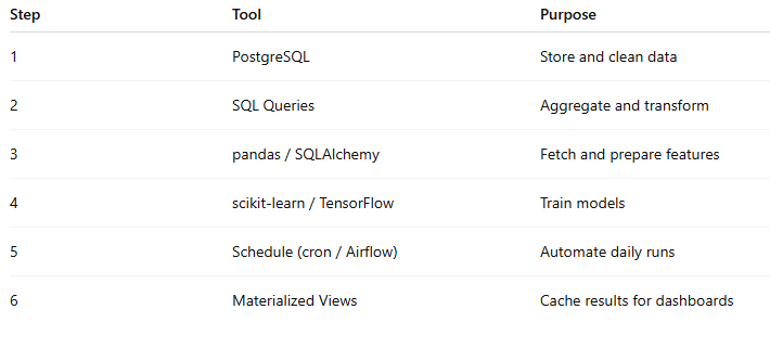
🧩 10 Practice Exercises

Connect to your PostgreSQL database using SQLAlchemy and print table names.
Use pandas to read 100 rows from a large table.
Write a new DataFrame into PostgreSQL with to_sql.
Run a parameterized query to filter users by city name.
Build an ETL job that extracts, transforms (normalize one column), and writes back.
Wrap multiple inserts in one transaction and test rollback on error.
Schedule a Python function to refresh a materialized view every hour.
Read a view into pandas and export it to CSV.
Use SQL + pandas to calculate moving averages and plot them.
Combine SQL (data extraction) and scikit-learn (regression model) end-to-end.

Chapter 12 — Final Project: End-to-End AI Data Pipeline

(PostgreSQL + SQL + Python + Feature Engineering + ETL + Automation)

🎯 Project Goal

This final project brings everything together into a real-world AI data pipeline, where:

Data is collected and stored in PostgreSQL.
SQL transforms raw logs into clean, feature-rich tables.
Python automates ETL and triggers model training.
The pipeline runs daily — automatically refreshing features.

By the end, you’ll have a production-style mini data pipeline, like what Data Engineers and AI Developers build in real jobs.

🧠 Project Scenario

You’re working for an AI-driven e-commerce platform called ShopAI.
You have two main datasets:

orders → every purchase made by a user.
users → information about customers.

Your job is to:

Clean and prepare this raw data.
Generate analytical features for churn prediction and spend forecasting.
Automate the pipeline using Python and schedule it daily.

📊 Database Setup (SQL Schema)

-- DROP old tables
DROP TABLE IF EXISTS users CASCADE;
DROP TABLE IF EXISTS orders CASCADE;

-- USERS TABLE
CREATE TABLE users (
  user_id SERIAL PRIMARY KEY,
  name TEXT,
  signup_date DATE,
  city TEXT
);

-- ORDERS TABLE
CREATE TABLE orders (
  order_id SERIAL PRIMARY KEY,
  user_id INT REFERENCES users(user_id),
  order_date DATE,
  amount NUMERIC(8,2)
);

🧩 Step 1 — Insert Sample Data

INSERT INTO users (name, signup_date, city) VALUES
(’Alice’,’2025-01-01’,’Paris’),
(’Ben’,’2025-01-03’,’London’),
(’Carmen’,’2025-01-05’,’Paris’),
(’David’,’2025-01-10’,’Berlin’);

INSERT INTO orders (user_id, order_date, amount) VALUES
(1,’2025-01-02’,100),
(1,’2025-01-05’,120),
(1,’2025-01-10’,80),
(2,’2025-01-04’,200),
(2,’2025-01-07’,150),
(3,’2025-01-10’,50),
(4,’2025-01-11’,300),
(4,’2025-01-14’,200);

🧩 Step 2 — Clean the Data

-- remove duplicates if any
DELETE FROM orders a USING orders b
WHERE a.ctid < b.ctid
  AND a.user_id=b.user_id
  AND a.order_date=b.order_date;

-- fix nulls with COALESCE
UPDATE users SET city = COALESCE(city, ‘Unknown’);

Why: ensures data consistency before analysis.

🧩 Step 3 — Generate Features (SQL Feature Engineering)

1️⃣ Total spend, average spend, last order date

CREATE OR REPLACE VIEW user_features AS
SELECT
  u.user_id,
  u.name,
  u.city,
  COUNT(o.order_id) AS total_orders,
  SUM(o.amount) AS total_spend,
  ROUND(AVG(o.amount),2) AS avg_spend,
  MAX(o.order_date) AS last_order,
  CURRENT_DATE - MAX(o.order_date) AS days_since_last_order
FROM users u
LEFT JOIN orders o ON u.user_id=o.user_id
GROUP BY u.user_id, u.name, u.city;

2️⃣ Add ranking per city (window function)

SELECT *,
  RANK() OVER (PARTITION BY city ORDER BY total_spend DESC) AS rank_in_city
FROM user_features;

🧩 Step 4 — Create Materialized Feature Store

DROP MATERIALIZED VIEW IF EXISTS user_feature_store;
CREATE MATERIALIZED VIEW user_feature_store AS
SELECT *,
       CASE
         WHEN days_since_last_order > 5 THEN ‘Inactive’
         ELSE ‘Active’
       END AS activity_flag
FROM user_features;

-- refresh manually when new orders arrive
REFRESH MATERIALIZED VIEW user_feature_store;

SELECT * FROM user_feature_store;

Purpose:
Materialized views store snapshots of features for faster model input.

🧩 Step 5 — Build Python ETL Script

# etl_shopai.py
import pandas as pd
from sqlalchemy import create_engine, text
import datetime

engine = create_engine(”postgresql://postgres:password@localhost:5432/ai_course”)

print(”🧩 Starting ETL at”, datetime.datetime.now())

# 1. Extract data
df_users = pd.read_sql(”SELECT * FROM users;”, engine)
df_orders = pd.read_sql(”SELECT * FROM orders;”, engine)

# 2. Transform (feature engineering)
df_features = (
    df_orders.groupby(”user_id”)
    .agg(total_orders=(”order_id”,”count”),
         total_spend=(”amount”,”sum”),
         avg_spend=(”amount”,”mean”),
         last_order=(”order_date”,”max”))
    .reset_index()
)

df_features[”days_since_last_order”] = (
    pd.Timestamp(”2025-01-15”) - pd.to_datetime(df_features[”last_order”])
).dt.days

# 3. Join with users table
df_final = pd.merge(df_users, df_features, on=”user_id”, how=”left”)
df_final[”activity_flag”] = df_final[”days_since_last_order”].apply(
    lambda x: “Inactive” if x>5 else “Active”
)

# 4. Load to PostgreSQL
df_final.to_sql(”user_feature_store_py”, engine, if_exists=”replace”, index=False)
print(”✅ ETL completed and stored in PostgreSQL.”)

🧩 Step 6 — Schedule Daily Feature Updates

You can schedule this ETL using Python’s schedule module or cron.

import schedule, time
from subprocess import run

def run_daily_pipeline():
    run([”python3”,”etl_shopai.py”])

schedule.every().day.at(”02:00”).do(run_daily_pipeline)

while True:
    schedule.run_pending()
    time.sleep(60)

🧩 Step 7 — Use Features in a Machine Learning Model

import pandas as pd
from sqlalchemy import create_engine
from sklearn.linear_model import LogisticRegression

engine = create_engine(”postgresql://postgres:password@localhost:5432/ai_course”)
df = pd.read_sql(”SELECT * FROM user_feature_store_py;”, engine)

# Example target: Inactive=1, Active=0
df[”target”] = (df[”activity_flag”]==”Inactive”).astype(int)

X = df[[”total_orders”,”total_spend”,”avg_spend”,”days_since_last_order”]]
y = df[”target”]

model = LogisticRegression()
model.fit(X, y)

print(”Model coefficients:”, model.coef_)
print(”✅ Model trained on SQL-generated features.”)

🧩 Step 8 — Monitor and Refresh

Set REFRESH MATERIALIZED VIEW user_feature_store; nightly in SQL.
Or schedule Python ETL to rerun daily.
Monitor data quality (check missing, anomalies).

⚙️ Full Pipeline Flow

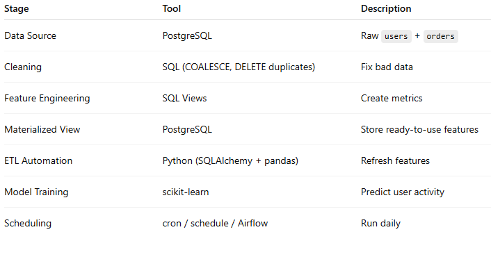
🧩 10 Practice Exercises

Add a refunds table and compute net_spend = total_spend - refunds.
Include a days_since_signup feature from the users table.
Rank users globally and per city.
Detect high-value customers (top 10% spenders).
Automate feature refresh every hour using Python’s schedule.
Add a daily anomaly detection query for negative order amounts.
Export final features to CSV for ML.
Visualize daily spend trend in Python with matplotlib.
Extend ETL to include new feature: “average gap between orders”.
Package ETL as a CLI command (python etl_shopai.py --refresh).

🏁 You’ve Completed the Full PostgreSQL + AI Data Mastery Roadmap 🎉

By finishing this course and project, you now understand:
✅ SQL for data retrieval and joins
✅ Advanced analytics (window functions, subqueries, aggregates)
✅ Data cleaning and optimization
✅ JSON/arrays and semi-structured data
✅ Python integration and ETL automation
✅ Full feature-engineering workflow for AI

🏆 10. Resume/Portfolio Description

Title: AI-Driven Data Pipeline with PostgreSQL and Python
Duration: 3 weeks
Tech Stack: PostgreSQL, SQL, Python, pandas, SQLAlchemy, scikit-learn, schedule

Description:

Designed and implemented an automated data pipeline that extracts transactional data from PostgreSQL, performs SQL-based feature engineering, loads cleaned data into a materialized view, and triggers Python-based model training daily. Included anomaly detection and activity segmentation features used for churn prediction.

Highlights:

Built ETL pipeline using pandas + SQLAlchemy
Created 10+ AI-ready features using SQL window functions
Designed automated feature refresh using Python scheduler
Trained ML model for churn prediction on SQL-generated features

💼 11. GitHub 🧪 Assessment (For Learners)

Students enrolled in the CareerByteCode AI Data Pipeline Course must use this repository as part of their practical assessment.

Objective:
Identify, debug, and fix small intentional issues in the project to gain real-world experience.

Git Repo : https://github.com/careerbytecode/ShopAI_Project.git

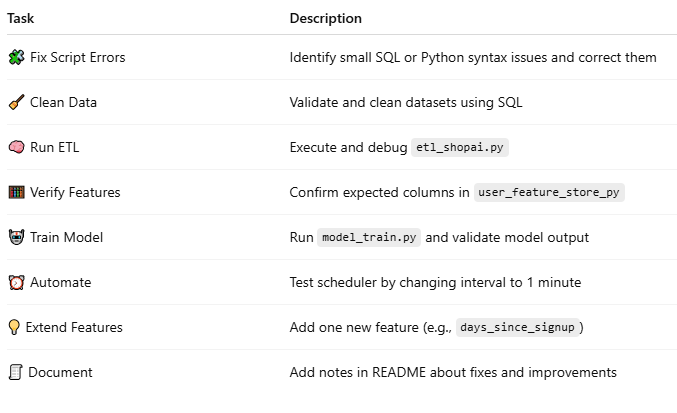
✅ Completion Criteria

You’ve successfully completed the project when:

All scripts and Python files run end-to-end without errors
user_feature_store_py populates correctly
Model trains successfully with visible coefficients
Scheduler triggers ETL automatically
You can explain every step (schema → ETL → model)

💡 Bonus Challenges

Create an additional materialized view that aggregates daily revenue
Add a plot or visualization of average spend per city using Python
Build a Dockerfile to containerize the project
Deploy the PostgreSQL + ETL pipeline using Docker Compose
Integrate with Grafana or Metabase for dashboard visualization

🧠 Learning Outcomes

After completing this project, you’ll master:

SQL for AI & Feature Engineering
Python + PostgreSQL ETL Automation
Data Cleaning and Quality Validation
Feature Store Design for ML Models
Automation and Scheduling Concepts

📘 Chapter 13 — PostgreSQL with Python (Integration)

This chapter teaches how to connect PostgreSQL with Python, run SQL queries programmatically, perform CRUD operations, handle exceptions, and integrate with libraries like pandas for AI workflows.

Each concept is explained in layman’s terms, includes 5+ runnable examples (with tables + data), and ends with 10 exercises for practice.

🎯 Goal of This Chapter

By the end of this chapter, you’ll learn how to:

Connect Python to PostgreSQL
Run SQL commands (SELECT, INSERT, UPDATE, DELETE) from Python
Handle database transactions safely
Fetch and process query results in Python
Use pandas + SQLAlchemy for data analysis and ETL
Build mini real-world examples (AI data preparation, feature extraction)

🧠 1. Introduction

PostgreSQL is a database system that stores and manages data.
Python is a programming language that can talk to this database to insert, retrieve, and analyze data.

To connect them, we use connectors like:

psycopg2 — The most popular PostgreSQL driver.
SQLAlchemy — A high-level ORM (Object Relational Mapper).
pandas — For data analysis and loading query results into DataFrames.

🧩 2. Installing Dependencies

Run these commands in your terminal:

pip install psycopg2-binary sqlalchemy pandas

psycopg2-binary: For connecting and running SQL queries
SQLAlchemy: For engine-based connections
pandas: For loading SQL query results into dataframes

🧩 3. Establishing Connection with psycopg2

Here’s how you can connect Python to PostgreSQL.

🧱 Example 1 — Basic Connection Test

import psycopg2

try:
    conn = psycopg2.connect(
        host=”localhost”,
        database=”ai_course”,
        user=”postgres”,
        password=”password”
    )
    print(”✅ Connection successful!”)
    conn.close()
except Exception as e:
    print(”❌ Connection failed:”, e)

Explanation:
This code connects Python to PostgreSQL using your credentials and prints success or error messages.

🧩 4. Creating a Table from Python

We can use Python to create tables dynamically.

🧱 Example 2 — Create Table “students”

import psycopg2

conn = psycopg2.connect(host=”localhost”, database=”ai_course”, user=”postgres”, password=”password”)
cur = conn.cursor()

cur.execute(”“”
CREATE TABLE IF NOT EXISTS students (
    id SERIAL PRIMARY KEY,
    name VARCHAR(50),
    age INT,
    marks NUMERIC(5,2)
)
“”“)
conn.commit()
print(”✅ Table created successfully”)

cur.close()
conn.close()

🧩 5. Inserting Data into Table

We can insert data directly from Python using SQL commands.

🧱 Example 3 — Insert Records

import psycopg2

conn = psycopg2.connect(host=”localhost”, database=”ai_course”, user=”postgres”, password=”password”)
cur = conn.cursor()

data = [
    (’Alice’, 22, 88.5),
    (’Ben’, 24, 92.0),
    (’Carmen’, 21, 75.0)
]

for row in data:
    cur.execute(”INSERT INTO students (name, age, marks) VALUES (%s, %s, %s)”, row)

conn.commit()
print(”✅ Data inserted successfully”)

cur.close()
conn.close()

🧩 6. Fetching Data from PostgreSQL

You can fetch data from PostgreSQL into Python using fetchall() or fetchone().

🧱 Example 4 — Read All Data

import psycopg2

conn = psycopg2.connect(host=”localhost”, database=”ai_course”, user=”postgres”, password=”password”)
cur = conn.cursor()

cur.execute(”SELECT * FROM students”)
rows = cur.fetchall()

for row in rows:
    print(row)

cur.close()
conn.close()

Output:

(1, ‘Alice’, 22, 88.5)
(2, ‘Ben’, 24, 92.0)
(3, ‘Carmen’, 21, 75.0)

🧩 7. Updating & Deleting Records

You can update and delete rows using Python queries.

🧱 Example 5 — Update Marks & Delete Record

import psycopg2

conn = psycopg2.connect(host=”localhost”, database=”ai_course”, user=”postgres”, password=”password”)
cur = conn.cursor()

# Update
cur.execute(”UPDATE students SET marks = marks + 5 WHERE name = ‘Carmen’”)

# Delete
cur.execute(”DELETE FROM students WHERE name = ‘Ben’”)

conn.commit()
print(”✅ Updated and deleted successfully”)

cur.close()
conn.close()

🧩 8. Using Pandas to Query PostgreSQL

You can load SQL results directly into a DataFrame using pandas.read_sql().

🧱 Example 6 — Load Table into pandas

import pandas as pd
import psycopg2

conn = psycopg2.connect(host=”localhost”, database=”ai_course”, user=”postgres”, password=”password”)

df = pd.read_sql(”SELECT * FROM students”, conn)
print(df)

conn.close()

Output:

   id   name  age  marks
0   1  Alice   22   88.5
1   3  Carmen  21   80.0

🧩 9. Using SQLAlchemy for Cleaner Code

SQLAlchemy allows connection reuse and ORM-like access.

🧱 Example 7 — Using SQLAlchemy Engine

from sqlalchemy import create_engine
import pandas as pd

engine = create_engine(”postgresql://postgres:password@localhost:5432/ai_course”)

# Read
df = pd.read_sql(”SELECT * FROM students”, engine)
print(df)

# Write
new_data = pd.DataFrame({’name’: [’David’], ‘age’: [25], ‘marks’: [89.5]})
new_data.to_sql(’students’, engine, if_exists=’append’, index=False)
print(”✅ Inserted using pandas + SQLAlchemy”)

🧩 10. Using Python + PostgreSQL for AI Use Case

Let’s simulate a mini AI data preparation example.

We’ll:

Store customer purchase data
Calculate average spend per user
Export clean data for model training

🧱 Example 8 — Mini AI Pipeline

from sqlalchemy import create_engine
import pandas as pd

engine = create_engine(”postgresql://postgres:password@localhost:5432/ai_course”)

# Create a table
with engine.connect() as conn:
    conn.execute(”“”
    CREATE TABLE IF NOT EXISTS orders (
        id SERIAL PRIMARY KEY,
        user_name TEXT,
        amount NUMERIC(8,2)
    )
    “”“)
    conn.execute(”INSERT INTO orders (user_name, amount) VALUES (’Alice’,100),(’Alice’,150),(’Ben’,200),(’Carmen’,50)”)
    conn.commit()

# Load into pandas
df = pd.read_sql(”SELECT user_name, AVG(amount) as avg_spend, SUM(amount) as total_spend FROM orders GROUP BY user_name”, engine)

print(df)

Output:

  user_name  avg_spend  total_spend
0     Alice      125.0        250.0
1       Ben      200.0        200.0
2    Carmen       50.0         50.0

🧠 11. Handling Exceptions and Transactions

Always use try-except-finally to avoid connection leaks.

🧱 Example 9 — Error Handling

import psycopg2

try:
    conn = psycopg2.connect(host=”localhost”, database=”ai_course”, user=”postgres”, password=”wrongpass”)
    cur = conn.cursor()
    cur.execute(”SELECT * FROM students”)
    print(cur.fetchall())
except Exception as e:
    print(”❌ Something went wrong:”, e)
finally:
    if conn:
        conn.close()

🧩 12. Real-World Data Integration Flow

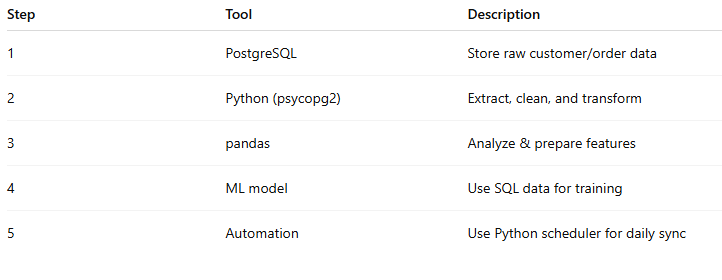
🧠 13. Summary

✅ PostgreSQL and Python work hand-in-hand for AI and data analytics.
✅ You can connect, query, clean, and transform SQL data in Python seamlessly.
✅ This integration forms the backbone of AI Data Pipelines.

🧩 14. Exercises

Try these for hands-on practice:

Create a new table employees (id, name, dept, salary) and insert 5 records.
Fetch only employees earning above a certain salary using Python.
Write a Python function that accepts user input and inserts data.
Write a query to find average salary per department.
Update all salaries by +10% using Python.
Delete employees with salary < 50000.
Fetch all rows into a pandas DataFrame.
Export DataFrame results to a CSV file using df.to_csv().
Handle invalid connections using try-except.
Create a simple dashboard (print stats) of department-wise salary spend.

📘 Chapter 14 — Data Warehousing & Analytical Extensions

🎯 Goal of This Chapter

By the end of this chapter, you will learn:

✅ What a Data Warehouse is and how PostgreSQL can act as one
✅ How to use advanced PostgreSQL features for analytics (CTEs, Materialized Views, Partitions, Window Functions)
✅ How to design star and snowflake schemas
✅ How to build and optimize analytical queries
✅ How to use extensions like cube, tablefunc, and pg_partman for analytics
✅ How to prepare aggregated data for AI/BI tools (Power BI, Tableau, Looker)

🧠 1. What Is a Data Warehouse?

A Data Warehouse (DW) is a central storage system used for analysis and reporting — not for frequent updates.

It’s different from a transactional database (OLTP).

Type Purpose Example OLTP Stores live, transactional data eCommerce order DB OLAP / DW Stores aggregated, historical data Reporting, analytics, AI model data

In AI/ML workflows, you typically:

Extract raw data from sources
Transform it (clean, aggregate, enrich)
Load into the warehouse
Query for analytics or feature generation

PostgreSQL can do all this!

🧩 2. PostgreSQL as a Data Warehouse

PostgreSQL supports:

Indexes for fast queries
Materialized views for snapshots
CTEs and window functions for analytics
Partitioning for large datasets
Extensions for advanced aggregation

Let’s simulate a small Retail Data Warehouse.

🧱 Example Schema: Retail Analytics

-- Drop existing tables
DROP TABLE IF EXISTS sales, customers, products CASCADE;

-- Dimension Tables
CREATE TABLE customers (
    customer_id SERIAL PRIMARY KEY,
    name TEXT,
    city TEXT,
    signup_date DATE
);

CREATE TABLE products (
    product_id SERIAL PRIMARY KEY,
    product_name TEXT,
    category TEXT,
    price NUMERIC(8,2)
);

-- Fact Table
CREATE TABLE sales (
    sale_id SERIAL PRIMARY KEY,
    customer_id INT REFERENCES customers(customer_id),
    product_id INT REFERENCES products(product_id),
    quantity INT,
    sale_date DATE
);

🧩 3. Insert Sample Data

INSERT INTO customers (name, city, signup_date) VALUES
(’Alice’,’Paris’,’2024-01-10’),
(’Ben’,’London’,’2024-01-15’),
(’Carmen’,’Paris’,’2024-02-01’),
(’David’,’Berlin’,’2024-02-05’);

INSERT INTO products (product_name, category, price) VALUES
(’Laptop’,’Electronics’,1200),
(’Phone’,’Electronics’,800),
(’Shoes’,’Fashion’,150),
(’Watch’,’Fashion’,300);

INSERT INTO sales (customer_id, product_id, quantity, sale_date) VALUES
(1,1,1,’2024-02-10’),
(1,3,2,’2024-02-15’),
(2,2,1,’2024-02-12’),
(3,4,1,’2024-02-14’),
(4,3,3,’2024-02-15’);

🧠 4. Star Schema Design

Your fact table (sales) links to dimension tables (customers, products).

Visually:

       customers        products
           \              /
            \            /
             \          /
              \        /
               \      /
                 sales (fact)

This is a Star Schema, ideal for analytical queries and AI feature generation.

🧩 5. Analytical Queries

Let’s see how PostgreSQL can be used like a warehouse:

🧱 Example 1 — Total Sales by City

SELECT c.city, SUM(p.price * s.quantity) AS total_sales
FROM sales s
JOIN customers c ON s.customer_id = c.customer_id
JOIN products p ON s.product_id = p.product_id
GROUP BY c.city;

Result:

city total_sales Paris 1650 London 800 Berlin 450

🧱 Example 2 — Top-Selling Product Category

SELECT p.category, SUM(s.quantity) AS total_quantity
FROM sales s
JOIN products p ON s.product_id = p.product_id
GROUP BY p.category
ORDER BY total_quantity DESC;

Result:

category total_quantity Fashion 6 Electronics 2

🧱 Example 3 — Monthly Revenue Trend

SELECT DATE_TRUNC(’month’, sale_date) AS month, 
       SUM(p.price * s.quantity) AS total_revenue
FROM sales s
JOIN products p ON s.product_id = p.product_id
GROUP BY month
ORDER BY month;

🧱 Example 4 — Cumulative Revenue (Window Function)

SELECT 
    DATE_TRUNC(’month’, sale_date) AS month,
    SUM(p.price * s.quantity) AS monthly_revenue,
    SUM(SUM(p.price * s.quantity)) OVER (ORDER BY DATE_TRUNC(’month’, sale_date)) AS cumulative_revenue
FROM sales s
JOIN products p ON s.product_id = p.product_id
GROUP BY month
ORDER BY month;

🧩 6. Materialized Views for Precomputed Analytics

Materialized views store snapshots of results — great for dashboards.

CREATE MATERIALIZED VIEW city_sales_summary AS
SELECT c.city, SUM(p.price * s.quantity) AS total_sales
FROM sales s
JOIN customers c ON s.customer_id = c.customer_id
JOIN products p ON s.product_id = p.product_id
GROUP BY c.city;

-- Refresh manually
REFRESH MATERIALIZED VIEW city_sales_summary;
SELECT * FROM city_sales_summary;

🧩 7. Using Partitioning for Performance

Partitioning improves performance on large datasets.

🧱 Example — Partition Sales by Month

CREATE TABLE sales_partitioned (
    sale_id SERIAL,
    customer_id INT,
    product_id INT,
    quantity INT,
    sale_date DATE
) PARTITION BY RANGE (sale_date);

CREATE TABLE sales_2024_01 PARTITION OF sales_partitioned
FOR VALUES FROM (’2024-01-01’) TO (’2024-02-01’);

CREATE TABLE sales_2024_02 PARTITION OF sales_partitioned
FOR VALUES FROM (’2024-02-01’) TO (’2024-03-01’);

Now:
When you query by WHERE sale_date BETWEEN ..., PostgreSQL scans only relevant partitions.

🧩 8. Analytical Extensions

PostgreSQL supports several extensions that make it behave like a true analytical engine.

🧱 Example 1 — `cube` Extension (for Multidimensional Aggregation)

CREATE EXTENSION IF NOT EXISTS cube;
CREATE EXTENSION IF NOT EXISTS earthdistance;

Use Case: Geographic distance calculations, multi-dimensional grouping (great for BI and ML features).

🧱 Example 2 — `tablefunc` (Pivot Tables)

CREATE EXTENSION IF NOT EXISTS tablefunc;

SELECT * FROM crosstab(
  ‘SELECT city, category, SUM(price * quantity)
   FROM sales s
   JOIN customers c ON s.customer_id=c.customer_id
   JOIN products p ON s.product_id=p.product_id
   GROUP BY city, category
   ORDER BY city’,
  ‘SELECT DISTINCT category FROM products ORDER BY category’
) AS pivot(city TEXT, electronics NUMERIC, fashion NUMERIC);

This transforms data into a pivot table (like Excel / Power BI).

🧱 Example 3 — `pg_partman` for Automatic Partition Management

Install:

CREATE EXTENSION IF NOT EXISTS pg_partman;

It automatically creates time-based partitions (daily/monthly).
Example: great for IoT or AI time series data pipelines.

🧩 9. Aggregation and Feature Store Use Case

In AI projects, we often convert raw tables into aggregated features (a mini feature store).

🧱 Example — Customer Feature Summary

CREATE VIEW customer_features AS
SELECT 
    c.customer_id,
    c.city,
    COUNT(s.sale_id) AS total_orders,
    SUM(p.price * s.quantity) AS total_spend,
    ROUND(AVG(p.price * s.quantity),2) AS avg_order_value,
    MAX(s.sale_date) AS last_order_date
FROM sales s
JOIN customers c ON s.customer_id = c.customer_id
JOIN products p ON s.product_id = p.product_id
GROUP BY c.customer_id, c.city;

Now this customer_features view can directly feed Python ML models for churn prediction or segmentation.

🧠 10. Data Warehouse Summary Query Patterns

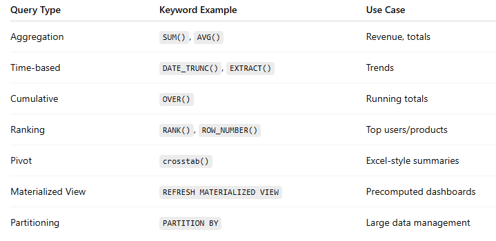
🧩 11. Exercises

Practice these to master PostgreSQL Data Warehousing:

Create a new table returns (sale_id, return_date, reason) and join with sales to calculate return rate.
Create a daily revenue materialized view and refresh it.
Use a window function to calculate 7-day rolling average sales.
Partition the sales table by city.
Build a pivot table showing sales per category per city.
Use DATE_TRUNC() to build a monthly sales trend report.
Add a feature view showing customer recency (days_since_last_order).
Integrate with Python using pandas to load aggregated tables.
Compare performance between partitioned vs non-partitioned tables.
Export analytical query results to a CSV for Power BI.

🧾 Summary

✅ PostgreSQL can be used as a full-featured analytical warehouse.
✅ Materialized Views, Window Functions, and Extensions power advanced AI pipelines.
✅ You can store aggregated, historical, and computed features directly in PostgreSQL.
✅ Python and BI tools can consume these features for dashboards or AI models.

🏁 PostgreSQL for AI/Data/ML – Course Summary & Certification Guide

🎓 Course Overview

This comprehensive 14-chapter program transforms learners from SQL beginners into PostgreSQL professionals ready for AI and Data Engineering roles.

Through this journey, you’ve covered:

Core SQL fundamentals
Analytical and AI-driven queries
Feature engineering concepts
Integration with Python
Data warehousing and performance optimization

Each topic was built progressively — connecting real-world data, AI problem-solving, and hands-on coding that works out of the box.

🧭 Full Course Path (All 14 Chapters)

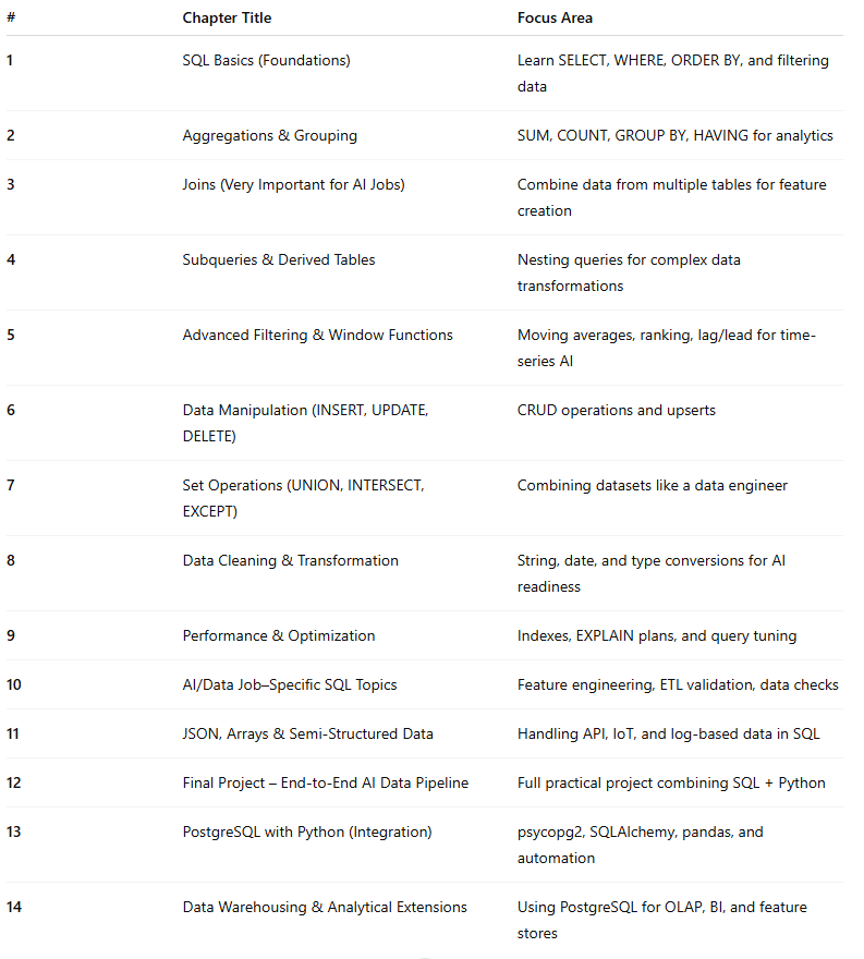
📊 Real-World Skills You’ve Gained

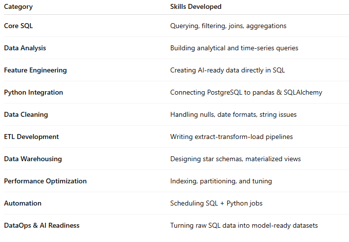
🧩 Project Recap – ShopAI Data Pipeline

You built (and/or debugged) a complete ShopAI Project integrating:

PostgreSQL schema design
ETL automation with Python
Feature store creation
Machine learning model integration
Scheduler for daily data refresh

This mirrors real-world AI pipelines used by data engineers and MLOps teams.

📘 Recommended Tools for Post-Certification Practice

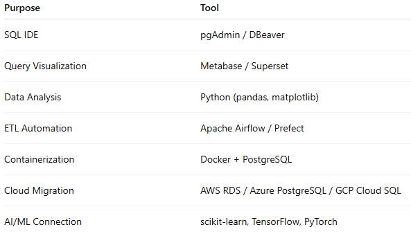
🧠 AI Career Application Areas

After mastering this course, you can confidently handle:

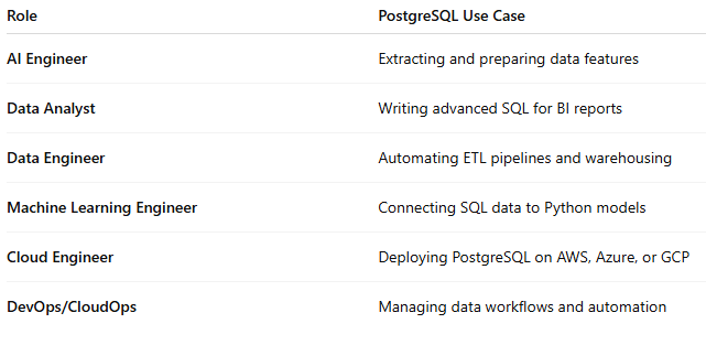
🧾 Certification Checklist

Before issuing your course completion certificate, ensure the learner has completed these 10 verifiable checkpoints:

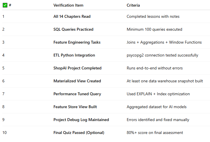
🏆 Certification Template (Example)

-----------------------------------------------
🎓 CareerByteCode | PostgreSQL for AI/Data/ML

This certifies that ___________________________
has successfully completed the 14-Chapter 
PostgreSQL for AI/Data/ML Program.

Skills Acquired:
✔ SQL Querying and Optimization
✔ Data Cleaning and Transformation
✔ Python Integration
✔ Feature Engineering
✔ Data Warehousing & ETL Automation

Date of Completion: ___________________________
Authorized by: ________________________________

CareerByteCode | Building AI-Ready Data Engineers
-----------------------------------------------

💬 Suggested Next Step (After This Course)

Once learners complete this PostgreSQL track, they can continue into:

Python for AI & Data Science (50 Projects Series)
Building Real-Time Data Pipelines with Airflow + PostgreSQL
MLOps Foundations: Deploying AI Pipelines on Cloud (AWS/Azure)
Power BI / Tableau Visualization with PostgreSQL Backends

🧭 Final Words

🎯 You’ve built a rock-solid foundation in PostgreSQL for AI and Data Engineering.
You now understand how to query, clean, model, and automate your data pipeline.

This knowledge bridges SQL and AI — empowering you to move confidently into Data Science, AI Engineering, or MLOps roles.

“The strongest AI models are built on clean, structured, and well-engineered data — and that’s exactly what you now know how to create.”

✅ Congratulations — You’ve Completed the Full PostgreSQL for AI/Data/ML Program!

AI & Analytics with PostgreSQL: Master Feature Engineering and Data Warehousing

💡 From Zero to Real-Time Analytics — Learn SQL the AI Way

🎯 Course Description

🚀 Who This Course Is For

📚 What You’ll Learn

📍 Foundations

📍 Intermediate SQL

📍 Advanced SQL

📍 Real-World AI Applications

🌟 Key Benefits

1️⃣ Real-World Ready

2️⃣ Python + SQL Integration

3️⃣ Practice Without Frustration

4️⃣ Visual Learning Approach

5️⃣ AI-Focused SQL Mastery

6️⃣ Practical Assignments

7️⃣ Career-Oriented Learning Path

🧠 By the End of This Course, You’ll Be Able To:

🕒 Duration

🧩 Course Structure

💼 Career Impact

🏆 Certificate of Completion

🚀 PostgreSQL Roadmap for AI / Data / ML Jobs

🔹Chapter 1. PostgreSQL Basics (Foundations)

🔹Chapter 2. Aggregations & Grouping

🔹Chapter 3. Joins (Essential for Data Engineering & AI)

🔹Chapter 4. Subqueries & CTEs (Common Table Expressions)

🔹Chapter 5. Advanced Filtering & Window Functions

🔹 Chapter 6. Data Manipulation

🔹 Chapter 7. Set Operations

🔹Chapter 8. Data Cleaning & Transformation (ETL Core)

🔹 Chapter 9. JSON & Semi-Structured Data (PostgreSQL Power Feature)

🔹Chapter 10. Array & Advanced Data Types

🔹Chapter 11. Performance & Optimization

🔹Chapter 12. AI / Data-Specific Use Cases

🔹Chapter 13. PostgreSQL with Python (Integration)

🔹Chapter 14. Data Warehousing & Analytical Extensions

✅ Summary: What You Must Master for AI Jobs

🔗 Recommended Tools for Practice

Chapter 1 — PostgreSQL Basics (Foundations)

What you’ll learn in this chapter (in one sentence)

Layman explanations (super simple)

Practical Examples (each is copy-paste runnable)

Example 1 — Basic SELECT and creating a table

Example 2 — Filtering with WHERE and operators

Example 3 — ORDER BY, LIMIT, OFFSET

Example 4 — Aliases, expressions, and casting

Example 5 — DISTINCT and basic uniqueness check

Example 6 — Basic table constraints (NOT NULL, UNIQUE, PRIMARY KEY)

Quick troubleshooting tips

10 Exercises (practice tasks for Chapter 1)

Chapter 2 — Aggregations & Grouping

What you’ll learn in plain English

Example 1 — Simple aggregates: COUNT, SUM, AVG, MIN, MAX

Example 2 — GROUP BY a single column: totals per category

Example 3 — GROUP BY multiple columns and time bucketing (DATE_TRUNC)

Example 4 — HAVING vs WHERE: filter groups (correct way)

Example 5 — COUNT(DISTINCT), FILTER clause, and conditional aggregates

Example 6 — NULLs, COUNT(*) vs COUNT(col), and grouping NULLs with COALESCE

Quick practical tips (layman)

10 Exercises — practice (all should be solved in PostgreSQL)

Chapter 3 — Joins (Very plain-English + runnable examples + 10 exercises)

What is a JOIN? (super simple)

Types of joins — in one line each

Syntax basics

Example 1 — INNER JOIN (basic)

Example 2 — LEFT JOIN (include unmatched left rows)

Example 3 — RIGHT JOIN and FULL OUTER JOIN

Example 4 — CROSS JOIN (cartesian product)

Example 5 — SELF JOIN (table joined to itself)

Example 6 — Multi-table joins (chain joins) + USING

Example 7 — JOIN with aggregate (which side to aggregate?)

Example 8 — JOIN pitfalls: duplicate join columns and ambiguous column names

10 Exercises — Joins (try them out)

Chapter 4 — Subqueries & CTEs (Common Table Expressions)

🧠 What You’ll Learn

🧩 1. What Is a Subquery? (Plain-English Explanation)

🧩 2. Subquery in WHERE (Find rows based on results of another query)

🧩 3. Subquery in FROM (Treat a subquery as a temporary table)

🧩 4. Subquery in SELECT (Compute an extra column)

🧩 2. Subquery in `WHERE` (Find rows based on results of another query)

🧩 3. Subquery in `FROM` (Treat a subquery as a temporary table)

🧩 4. Subquery in `SELECT` (Compute an extra column)

🧩 6. `EXISTS` vs `IN`

🧩 7. Common Table Expressions (CTEs) — `WITH` clause

🧩 Example 2 — Understanding `EXPLAIN`